The longitudinal dynamics analysis deals with the straight movement of the vehicle. Hence this define the equations which explain the driving, braking and reverse vehicle movement. This article summarize the main concepts, theories and equations for the straight forward path.

Before the calculation it is required the stablishment of the main assumptions are:

• Rigid wheels;
• Non variation of the wheelbase;
• The slope angle of the surface is constant.

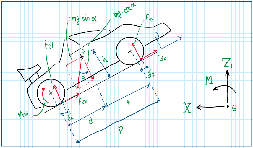
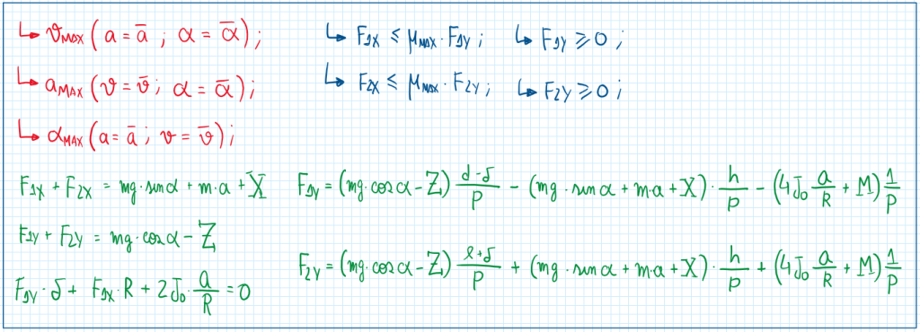
As can be seen the movement of a vehicle on the straight path is dependent of the following parameters F_1X, F_1Y, F_2X, F_2Y and M_m. The graph above illustrates all the effects that occur when I vehicle is traveling in a straight line. In addition it also accounts the aerodynamic forces which are translated to the center of gravity of the vehicle. Hence, Z represents the lift produced by the aero effects, M is the pitch moment due to the aero effects and X is the drag produced by the air resistance. Each of them depends of a relative velocity vr and air density. The analysis must also account the effects of loads and inertia of the tire/wheel. However, tires and wheels must be considered a rigid unique body which is not a correct approach as the tires are flexible and have a nonlinear behavior.

Equilibrium equations

To write the equilibrium equations it is important to account the external effect which are given by the drag, the lift and the pitch moment due to the aerodynamics.

The second step is to evaluate each wheel as the entire axle, thus both tires will be represented by just one theoretical tire with the values multiplied by two.

Taking advantage of the here tire contact points and using it as a reference it is possible to do the sum of all the equations. An important assumption is to consider the delta1 and delta2 (delta is rolling resistance coefficient) equal, this means that the tires are equals and their rolling resistance are also equals.

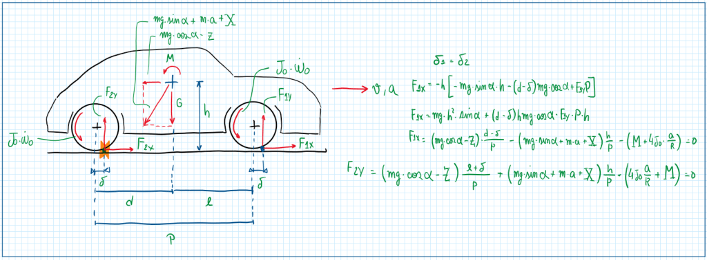
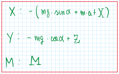
Therefore the five equilibrium equations for straight line movement can be written:

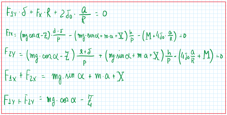
These equations that accounts the effects of the tires and the external loads. There are important assumption that about them:

• The tractive force of the tire cannot exceed the maximum friction capacity of these ones.
• The vertical reaction on the tires must not be negative which would mean that the surface is acting on the tires.

Now the longitudinal dynamic analysis will be concentrated on wheels. In the automobiles the wheels can be tractive or non-tractive. The first one exert torque to move the vehicle and the non-tractive just rolls and accounts negatively.

Tractive wheels

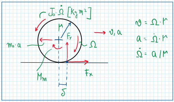
Hence considering a tractive wheel, the equilibrium equations are:

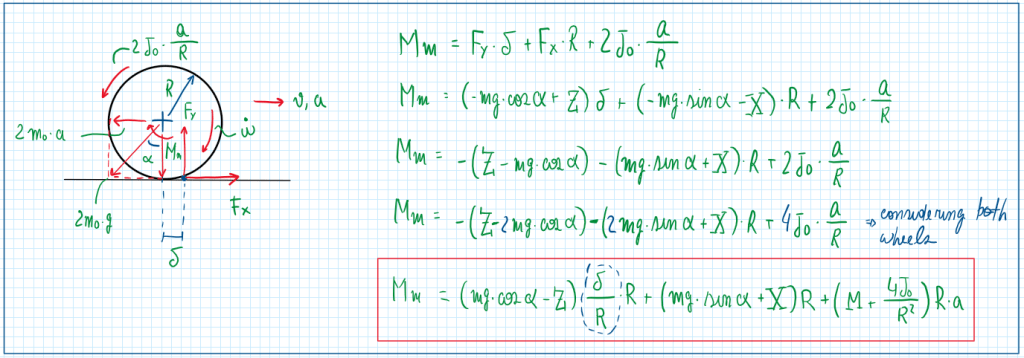
As can be observed on the picture, the tractive will account all the loads on the vehicle for the determination of the engine torque M_m. The forces F_X in F_Y only arise on the tractive wheel . Thus the non tractive wheels account negatively on the tractive one do it to their extra inertia component. In addition, all the aero force components were accounted and must be overcame by the engine torque. Relative to this one, the main term is the one given by delta divided by R, which is the rolling resistance. This is a normalized coefficient, because it is divided by the wheel radius R. This parameter can result on the following relation:

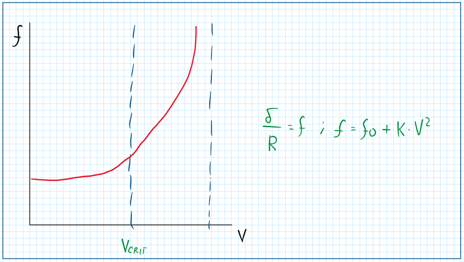
In general the parameter f has a value about 0.01 for asphalt or concrete surfaces . However this parameter is not constant and varies proportionally to the square of the velocity and the rate of increase is given by the coefficient K. Observing the graph, the increase occurs almost linearly until a point, which due to an error, the F increases abnormally. This point is given by the critical velocity, V_crit. Therefore the tire operation can only be made under the speed limit (V_crit), beyond this vibrations and waves propagates over the tire contact patch until a collapse.

Remarks about about friction coefficient and rolling resistance

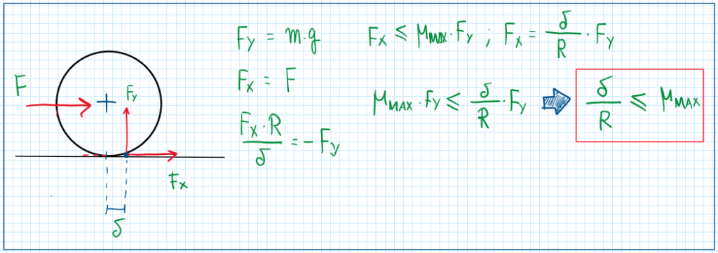
There are some considerations about the rolling coefficient and friction coefficient. In fact considering a wheel and establishing the following assumptions it is possible to write. As can be seen, the ratio between delta and R is less or equal to the maximum friction coefficient, which means that the rolling resistance coefficient cannot exceed the maximum friction coefficient. On the contrary, the wheel is unable to rotate. A situation which this usually happens are on off road conditions, more precisely on sand roads, which the values for the rolling resistance coefficient usually exceeds the maximum friction coefficient. Hence, the wheels slip over the surface without a pure rolling condition , in other words a rotation velocity different of the linear velocity of the wheel.

Non-tractive wheels

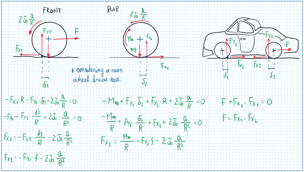
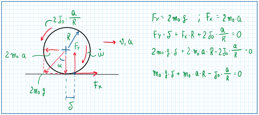
In the Figure above can be seen the force F required to overcome all the loads and the inertia of the attractive wheels must also deal with the rolling resistance and the inertia effects from the non-tractive wheels. In fact, non-tractive wheels consume grip from the attractive ones, thus reducing their traction performance. Using the equilibrium equations is possible to analyze some different the behaviors of the vehicle during a straight line traveling. First assuming a vehicle with rear wheel drive:

From these equations it is established a situation which a vehicle is traveling at low and constant speed, but the surface slope is the maximum value that the vehicle can overcome. Therefore the assumptions and equations are:

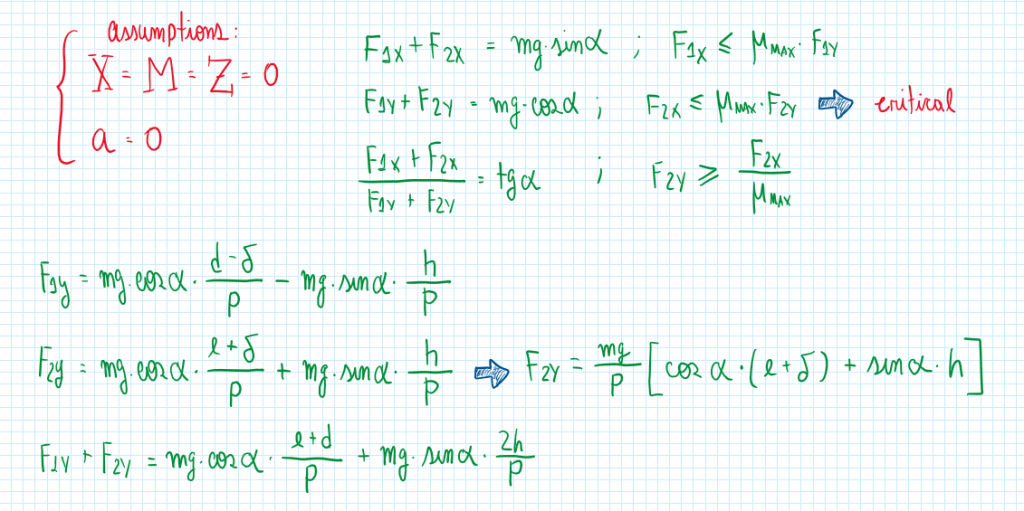
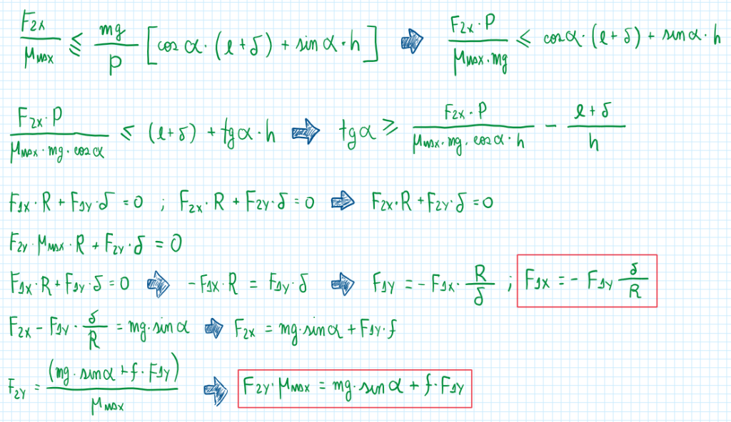
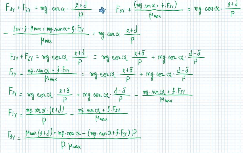
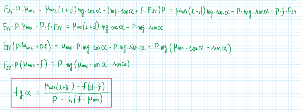
After all these calculations it is possible to conclude that for a low and constant speed in a inclined surface. The maximum slope possible for this vehicle depends of the tire capabilities, the weight partitioning and the rolling resistance coefficient.

References

• Guiggiani, Massimo. The Science of Vehicle Dynamics. Handling, Braking, and Ride of Road and Race Cars. New York, Springer, 2014;
• GILLESPIE, Thomas D, Fundamentals of Vehicle Dynamics, Warrendale, Society of Automotive Engineers, 1992. 470p.