This is the tire model which is simply used due to the assumptions made for it. In fact, precision of the results are not the aim, but what these results means follows what really happens with the tires. Hence, the brush model is qualitatively feasible. The figure above illustrates from what the model are composed. As can be noticed, the contact patch is perfectly symmetric and exhibits two distinct characteristics. First, the surface is squared and, second, the pressure curve on the tire admits a parabolical shape. The contact between tire and ground is made through bristles, they are infinitely thinner and their flexibility can be accounted longitudinally and transversally. In addition, the tire is considered a rigid and thin disc.

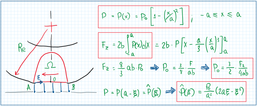
These three last equations (red square) describes that on brush models, the parabola shape gives a variation of the force and pressure along the x-direction. Hence, the pressure distribution and force resultant depends both of a nominal pressure P0, which is usually assumed as the same as the tire internal pressure. Although this system do not reproduce quantitatively what happens on real tire, the force  resultant equation can be adjusted by setting specific values in the place of 3/2. Considering that the system is modeled for a pure rolling conditions, it is required to establish some conditions:

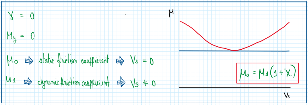
As can be seen, there is a short period which the friction coefficient reaches a value lower than usual and touches on the nominal line of the model. However, when this value became excessively high, the mu increases again. In general, the friction coefficient developed in a dynamic case follows a small relation between its value and the coefficient X, which is usually values about 0.20.

Bristles model

In general, the values for t oscillates around 30 and 60 MN/m², which are not so far from the characteristics. In fact, the tangential stiffness of the bristles can reproduce the real characteristics of the tire contact patch. Due to their flexibility, the tangential stress accounts both longitudinal and lateral effects.

Bristles modelling

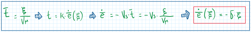
As can be seen, the tangential displacement of the bristles tips is a linear relation of the theoretical slip coefficients, in other words, it is connected to the speed of the wheel when slipping without slippage, in fact, is a ratio. The sign is the opposite of the theoretical, thus it is usually against the wheel motion. The only limitation of the bristle tip displacement is the friction coefficient produced between tire and ground. The bristle behave differently according to the following conditions:

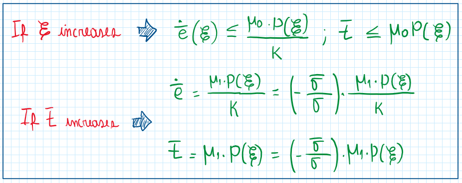
Conditions for the linear behavior

The conditions for the tangential stresses can be established:

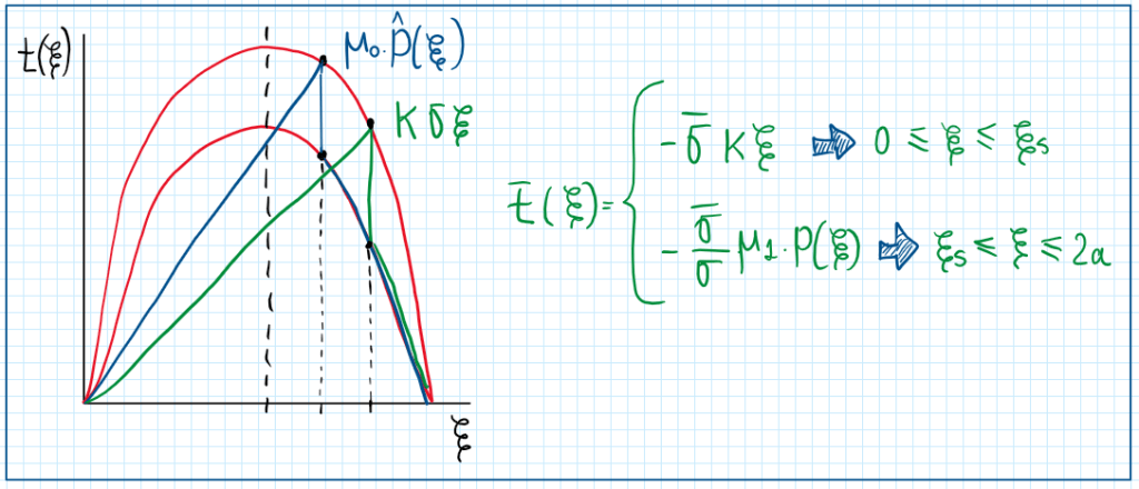
The graph illustrates the conditions which the linear behavior begins, at the beginning of the tire contact patch until epsilon, which becomes 2a. This is the total length of the tire contact patch. When epsilon becomes 2a, the total area was consumed by the slippage and then the tire is under unstable condition. However, the graph also exhibits that it is possible to change the path which this area will be vanished. In fact, this can be done by increasing t(epsilon) or epsilon. The stress on the contact patch is related to how much is the pressure distribution. A reduction of it makes possible to follow another path, in other words, another parabola. This can be described by the following equations:

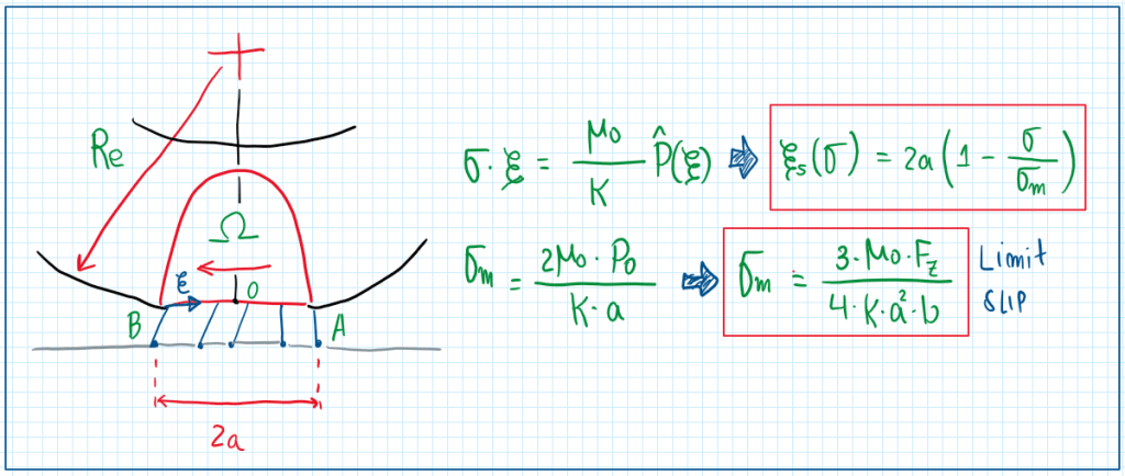
Hence, as can be seen, the value of sigma approximates to sigma_m, which is the limit slip. The value of epsilon_s represents the contact patch length which is being vanished by the slip condition. As epsilon_s goes from 2a until zero (point A), the contact patch is being splitted in a section with slipping and in another one with sticking. Therefore, when epsilon_s equals 2a, sigma became zero and when epsilon_s became zero, thus sigma became zero and when epsilon_s became zero, sigma equals sigma_m, unstable.

Tire with rectangular contact patch

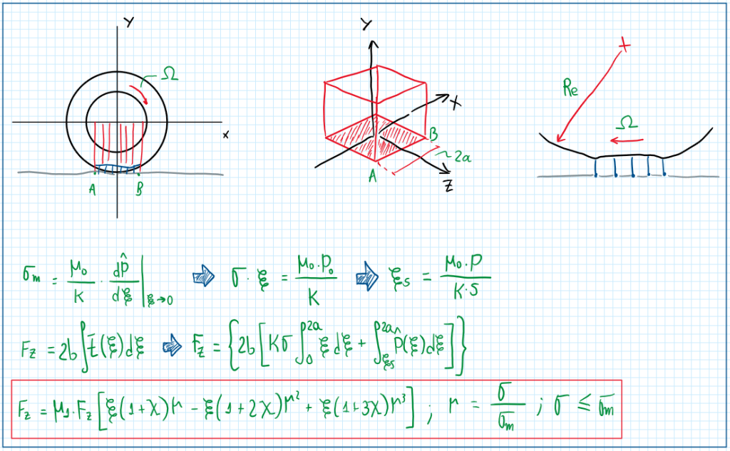
The total force on a rectangular contact patch is a function of the slip coefficients, which are contained in a power of three. In the same way, it is limited by sigma_m. In addition there are also the terms epsilon and X. The first is the auxiliary coordinator which determines how much the contact patch is on slip condition. The term X is the same as for the parabolic contact patch, but with different value. However, for the rectangular contact patch, there are two limiting conditions whose are given by:

The last two correlations are the classic theory of friction.

Example

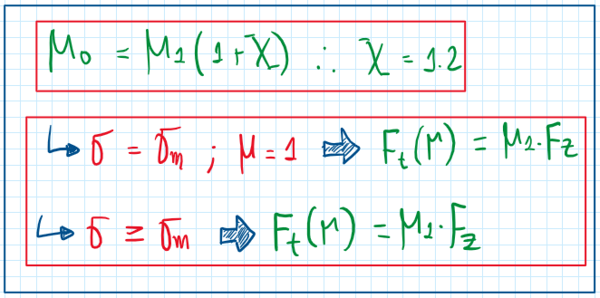
In this example, the total force is derived in terms of r tending to zero, thus the value of sigma_p is obtained. There are two X coefficients which can be used, 0.2 and 1.2, they represent parabolic distribution contact patch and the rectangular ones, respectively. The tires always operate under a certain degree of slip, this deals with the centrifugal force produced. In the absence of slip, part of the force produced by the tires are used to deal with the centrifugal force, thus a lower amount is able to handle longitudinal and lateral loads. Hence, tires require a certain amount of slip to work properly. However, from a specific point, the total force produced begins to decrease. Hence it is clear that if the theoretical slip coefficient is increasing, reduces Ft, which begins to be constant or, a locked conditions of the wheels.

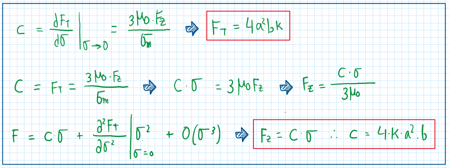
C coefficient

The graph and the expressions above suggest that, mu_max is not the maximum friction coefficient developed. This can be a bit counter intuitive, but mu_1 and mu_0 are coefficients which variates due to the conditions of the tires. As these represent extreme conditions, for instance, full grip or full slip, the maximum friction coefficient (mu_max) is the one which provides the best performance of the tire. Hence, the c coefficient can be calculated.

Therefore, it is now described that both total and vertical forces (Ft and Fz) are not only dependent of the theoretical slip coefficient, but also from the structural characteristics of the tires. However, this linearization is only beneficial when the forces are on the linear part of the curve. After this point, this assumption doe not reflect this tire condition anymore. In addition, it is important to mention that the tangential force direction is always the opposite one for the slip coefficient.

Therefore, for a case with T equal to 0, Fx is equal to 0 and sigma_x is equal to 0, thus Fy equals Ft.

References

• Guiggiani, Massimo. The Science of Vehicle Dynamics. Handling, Braking, and Ride of Road and Race Cars. New York, Springer, 2014;
• GILLESPIE, Thomas D, Fundamentals of Vehicle Dynamics, Warrendale, Society of Automotive Engineers, 1992. 470p.