The brush model is based in an one dimensional wheel rounded by bristles which touches the road. In addition these are allowed to deflect and deform its length. The bristles carry some important characteristics of the tire material parameters. There are two main situations used to study the tire behavior through the brush model, the pure rolling and the non-pure rolling. These are given by the formulas in the Figure 1. Hence, a pure rolling means that the tread elements remain vertical and move from the leading to the trailing edge. The non-pure rolling means that the rolling radius R_e is different for the translational wheel speed. This is the point which the tire generates friction and the bristles develops forces. There are three assumption taken by the brush model:

• The deflection vector does depend solely on the shear vector;
• The bristle stiffness is a scalar proportion between strain and stress;
• The relative speed V_S is parallel to the force generated by the tire.

As can be seen, bristles are more deformed at the leading edge, but when a slip angle α is applied, this deformation is combined with a lateral deformation. V_x is the longitudinal speed component while V_r is the longitudinal speed relative to the effective rotational radius. Hence, the following situations can be evaluated:

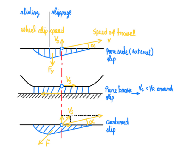
The first situation in the Figure 2 is the pure lateral slip (first graph at the top). The top view illustrates that α is the deviation of the speed of travel V from the tire center line. Hence, V is a vector that creates two components, the slip speed V_s and a longitudinal speed parallel to the tire center line. The second situation, is the pure braking slip, which is the graph at middle that illustrates the sideview of the tire. In this case, V_s is lower than V_r. However, V_s mentioned in this case is the longitudinal slip. It is also possible to visualize the braking force produced at the opposite direction relative to the movement. The third case illustrates the top view of the tire and what happens when there is a combined slip occurring. This situation can occur with the combination of acceleration and lateral loads or braking and lateral loads together. As can be seen, V_s is not anymore a vector of the traveling speed. Actually, V_s is always parallel to the force F generated by the tire. Hence, the angle of the relative speed V_s will be different from α, in this case. Two important conclusions that can be made after the analysis of these situations, is the slip coefficient for the case of braking and accelerating, the theoretical and the practical slip coefficients, respectively:

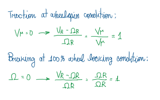
According to Figure 3, the relative speed V_s is equal to the rolling speed V_r. By Figures 1, 2 and 3 it is also possible to observe that, the bristle have their root fixed at a structure assumed as the tire carcass, while the tip of the bristle represent the tread. Hence, the bristle root has a relative movement respective to its tip. This increases from the leading to the trailing edge until the bristle detachment from the surface. In fact, the brush model assumes that only the tread is compliant and this is represented by the bristles. Any other tire component is assumed rigid.

If compared with other tire models, as beam, Fiala and Paceijka Magic Formula, the brush model is the one that produces the lowest results (Figure 4). In fact, quatitatively, this model is not suitable, but qualitatively is one of the bests, because it is one of the few models that correlates material properties with performance parameters of the tires. The brush model is a good representation if the tread and belt deflection are considered as one component.

Hence, the length of the bristle is the same, but with a lower stiffness. In fact, the choice of the material affects the belt, while the choice of the rubber compound affects the tread stiffness and characteristics.

Brush model contact patch distribution

The brush model collapses the contact patch into a line. However, it is assumed that the contact pressure is constant on the lateral directions, but changes along its length (Figure 6). Hence, F_Z will be a function of dY.

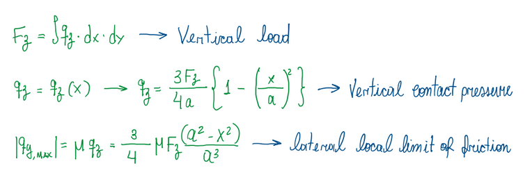
Hence, the contact pressure is just a parabolic distribution along the x-direction and the local friction shear stress will be defined by μ*q_z (Figure 7). Below this threshold, it is just a function of the material properties of the bristles.

Lateral slip

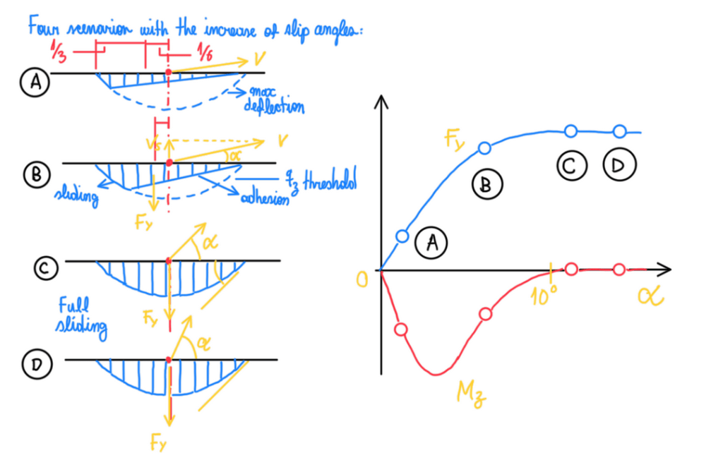
As can be seen, there are four situations, A, B, C and D, which α is being increased (Figure 8). At higher α values, some portions of the contact patch begin to slide. Hence, the slip region becomes smaller as the slide region becomes bigger. Increasing further α results also in the increase of the shear forces, but until some point. This is a threshold value which q_y = μ*q_z. After this, the tire is at full sliding condition and the peak of grip is reached. Therefore, the tire generates its maximum grip at full sliding condition.

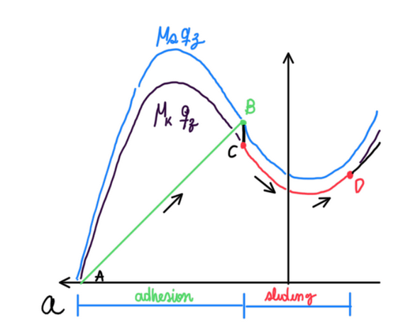
The critical point, is the transition of the situation B to C (Figure 9), because is not only the passage from the adhesion mechanism to the sliding one. Actually, is the transition of the static to the dynamic friction coefficient, μ_s to μ_k, respectively. Hence, this is the reason of the decay seen in the Figure 9, which characterize a real tire curve. It is possible notice that at a small α there is a condition of infinite μ, which means the adhesion condition, no slide. Therefore, the travel velocity can be calculated by the following formula:

It is interesting to observe (Figure 10) that it was started from combined slip condition and evaluated F_Y and M_Z in function of cp_y, which is the lateral stiffness of the bristles per unit length. At these two first formulas it is possible to visualize the main advantage of the brush model, the combination of contact patch area, α and cp_y. In other words, the dimension of the contact patch, speed (from α) and material properties of the tire tread, a connection with the main tire parameters. When these are partially derived by α and these tends to zero, it is possible to obtain the cornering stiffness C_Fα and the moment stiffness C_Mα , respectively. Another interesting detail about the brush model is the possibility to perform a stress-strain analogy:

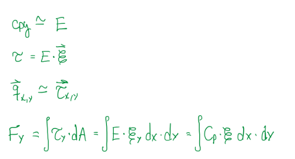
cp_y is equivalent to the Young’s modulus, the shear stress τ is equivalent to the local shear stress q_xy (Figure 11). Hence, q_xy is proportional to cp_y and the ratio between these two is equivalent to the shear strain ε. Therefore, the shear force formula can be updated for the lateral force one, which is now dependent of the contact patch area (dx*dy), ε and C_P (another notation for cornering stiffness). Another case of the brush model, is the finite μ or high slip and in this one it is possible to visualize that the stress-strain analogy is coherent.

Hence, at the threshold point, which is the transition between the linear and the parabolic behavior of the tread (Figure 12), it is possible to visualize that as α increases, the point in the Figure 10 goes more and more to the trailing edge. Therefore, the peak of grip represents that all points like that one are in the sliding condition. To find the intersection between linear and parabola the procedure is:

Hence, at the intersection point between these two conditions, the linear and the parabolic distribution are equivalent (Figure 13), thus writing q_y equals q_ymax it is possible to find:

θ_y is the composite tire parameter, it includes all the main tire factors (Figure 14). Since this condition, finite μ or high slip, represents the beginning of the sliding, it is correct to say that α, at this condition, is the one of the start of sliding, given by 1/θ_y. This is the first point at the contact patch that describes that the rubber reached its friction limit. This parameter is the another example that brush model is qualitatively good due to the correlation between the main factors of a tire. For the analysis of M_Z, it is possible to observe that:

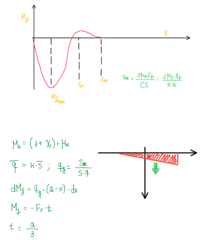
Hence, it is possible to conclude that assuming μ_s to μ_k by the correlation written above, M_Z behaves as illustrated by the Figure 15. The decay occurs due to the transition to μ_k. Hence, S_m describes better this case. In the case of constant μ, the behavior of M_Z is more predictable as seen in the Figure above. In addition, it is also possible to understand why the pneumatic trail is 1/3 of the contact patch length. Therefore, summarizing the equation for the brush model F_Y, M_Z and t:

All these parameters (Figure 16) can be visualized relative to the α in Figure 17:

As can be seen, M_Z, F_Y and t are normalized by similar parameters. From the Figure 17 it is possible to conclude that, when F_Y reaches the peak, M_Z and t are zero. Hence, the steering effort felt by the driver at this condition is just the mechanical trail. This occurs at a slip angle called, starting of sliding slip angle, given by 1/θ_y. The pneumatic trail t is at maximum when there is no F_Y, or rather, no α. Hence, t is basically connected to α. M_Z reaches its peak during linear phase of F_Y, around a α = 1/4θ_y. Usually, the cornering stiffness at F_Y(M_z at the peak) linear phase is about the arc tangent of 3θ_y.

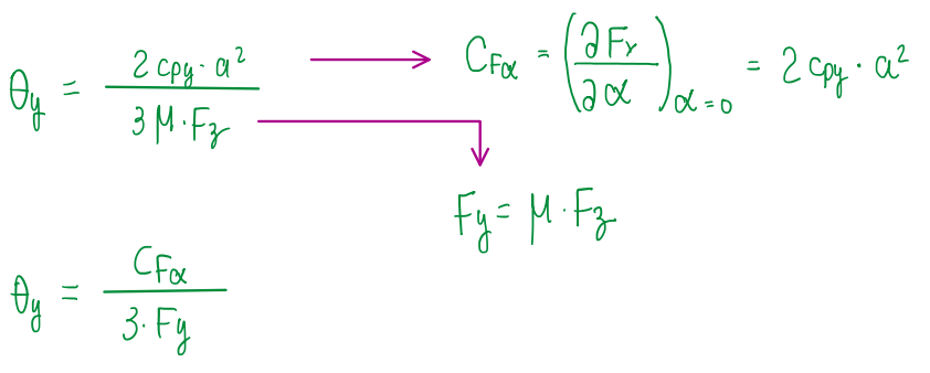
As can be noticed, all these parameters are referred to the composite tire parameter θ_y, which correlates the material properties of the tire tread and the lateral load. This is the power of the brush model, the only tire modeling that correlates the performance parameters with the material parameters. θ_y is basically a division of the cornering stiffness by three times the lateral load (Figure 18).

References

• Race Car Vehicle Dynamics – Miliken & Miliken;
• Guiggiani, Massimo. The Science of Vehicle Dynamics. Handling, Braking, and Ride of Road and Race Cars. New York, Springer, 2014.