Assuming a lap and the most critical situation at this one, it is possible to evaluate the fatigue stress and safety factor for many components of a race car. Some of them is not so complex, as the wheel hub, but components as the uprigh requires another technique Actually, when the number of cycles can not be precisely defined, the it is possible estimate through the variable amplitude loading (VAL) technique. In addition, with these data it is also possible to calculate the damage accumulation. This article proposes a brief review of these techniques applied for race components, as wheel hubs and uprights.

Wheel hub safety factor calculation

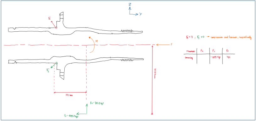
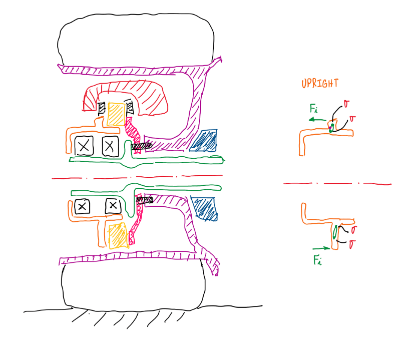
There are forces coming from the four wheels during a lap. The most critical one is taken and the point of the track which it happens is verified, usually a pure cornering situation. Figure 1 illustrates that wheel loads affects not only wheel hubs, as uprights and wishbones. Hence, this analysis begins with the simplest component, the wheel hub. Since the component in discussion is the hub, it is possible to simplify it in a cross-section:

Understanding that the hub is a rotating component, the stress at the point 1 and 2 will oscillate to an extreme positive and negative values (Figure 3).

Here, at a first approximation it is concentrated in the most critical maneuver. After defined the number of cycles, first apply the classical method. With this method is possible to separate the oscillating from the constant component. In addition, the notch effect is also accounted to take the damage accumulation. This is the main reason to use the Haigh equation (Figure 4).

Obviously eliminating conditions which are not critical:

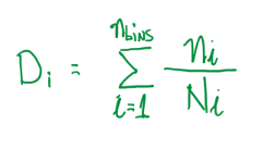
Where n_i is the cycle of the component when under operation, while N_i is the number of cycles referred to the material. Hence, when the damage accumulation D is applied, its value is lower than 1, this means that, considering a race car example, it will break before the end of one lap, or one race or a couple of races. Depends of what the number of cycles are being converted. After consider the value of D, it is possible to find the number of cycles:

In this case, Figure 6 illustrates that, even though the stress σ** is lower, it still will have some fatigue, because the number of cycles is higher. Therefore, the segment which the load occurs is segregated. Considering that the vehicle is under this condition and at constant regime, the amount of cycles calculated is defined and converted in mileage, but without the percentage of segment of the lap. Although, this suggests that velocity does not means a high stress, instead the frequency does. The stress components do not change. The next step is the application of the techniques in case of variable amplitude loading.

Upright safety factor calculation

The problem with component as the upright is that differently from wheel hubs, it does not rotate. Hence it is more difficult to estimate the number of cycles that it would support. However, there are tecniques to deal with this. In fact, this is the same variable amplitude loading (VAL) applied to the wheel hub, but adapted to the conditions of the upright. Another point that makes the upright safety factor calculation is that there many points in its geometry that can be considered the most requested one. Therefore, the first step is to acquire some data about the vehicle operation. This is obtained by data acquisitions systems and can be extracted to be used as reference.

Figure 8 illustrates the wheel loads over the time of operation. As can be seen, there is no trend or oscilatory pattern as in the wheel hubs (Figure 3 and 4). Hence the strategy is similar of the wheel hubs, take wheel loads cycles, split them in sections and apply a cycle counting technique. This evalutes the cycles even though they have completely different amplitudes.

One of the cycle counting techniques adopted is the Rainflow approach. By this one it is possible to identify which is the mean stress component σ_m and the local stress σ_a. Since the material is usually knon, the ultimate tensile strength R_m is given and by the Haigh equation it is possible calculate the safety factor. In addition, the Rainflow approach also allows to calculate the damage accumulation of the component. This and Raiflow technique will be discussed in the next topics.

The variable amplitude loading (VAL)

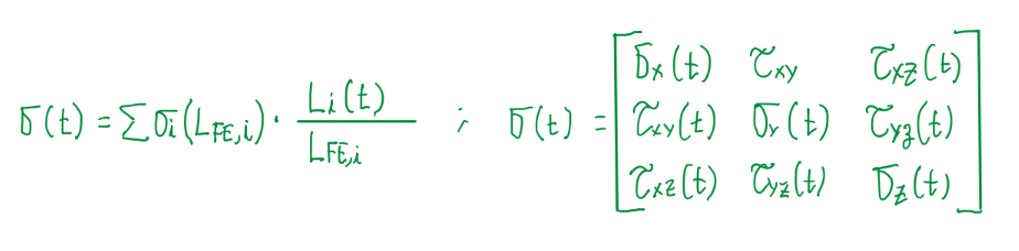
In the racing field data acquisition systems shows that in just 1 lap around a circuit, the chassis is submitted a very complex loadings. For fatigue analysis, loadings are not the parameter of interest, thus these are converted into stresses. Usually stresses are analyzed in terms of cycles. However, for so unpredictable loading case, the analysis is done in the time domain. Hence it is generated a stress-time series diagram. Since there are multiple loads acting, the time varying stress tensor σ(t) is generated:

Fatigue stress determination

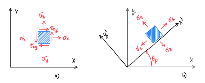
In some theoretical examples the fatigue calculation take into account the stress component σ_x. This is a straightforward procedure when the coordinate system is conveniently oriented in relation to the fatigue critical location (Figure 11). However, in real analysis this could not happen. Hence it is applied the Von Mises theory for principal and maximum shear stress.

Since the common application of Von Mises only accounts the range calculated from the positive load history, neglecting the negative part of the stress cycles, usually it is applied the signed Von Mises version of the original theory.

Hence, it us accounted both positive and negative stresses. Finally, the principal stresses for two dimensional analysis can be given by:

However, for three dimensional cases the approach is different. It is used the eigenvalues of the stress tensor for each time step:

The principal stresses, as seen above, are arranged by their algebraic value order. Since the principal stresses alone are not adequate for fatigue calculations, it is defined largest one according to the condition previously established.

Cycle counting

The main problem in multiple loads distribution is to perform the counting cycles, because there is no clear cycle occurring in the signal. Three techniques were proposed to count cycles, the reservoir, the rainflow and the binning methods.

Rainflow counting

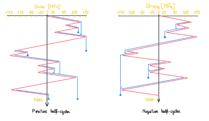
When the loading case is a very long time event, the best approach is the rainflow counting. Some literatures suggests to rotate clockwise the graph, others apply the method with the graph in its original position. In any case, the procedure is the same. First, count the positive half-cycles and then the second half-cycles. For the positive counting, the drop is stopped if it passes a more negative valley than it started. There cases which the drop stops when it encounters the run of existing drop. Figure 16 illustrates both cases. The negative one has the same approach. The main difference from the reservoir approach is that neither all cycles can be paired together. As can be seen, there are drops which are not paired. For these there are two options, or be considered as residual damage, or they can be closed together with the other drops to form a complete cycle.

Binning

After the counting process, the data generated is organized in a process called binning. This build graphs and histograms that describes the spectrum of the loading distributions (Figure 17). The values exhibited in these graphs are summarized by the Markov matrix.

Damage accumulation

All these procedure previously explained prepare the data to be used in the damage accumulation rule proposed by Palmgren-Miner, which is the fraction of the life consumed by a stress cycle with range delta σ_i, also defined previously.

Where Ni is the number of cycles at the given stress range and the associated mean stress range, σ_m,i.

The damage accumulation rule splits the load stores in groups with a specified stress range, which illustrated in Figure 19 as Δσ_q. Each group longs for an specified number of cycles, which is given by n_q. Hence, the damage accumulation rule can be updated to a more convenient form:

Each of these groups are summed to deliver the total damage factor, which usually ranges from 0.1 to 10 in real applications. However, theoretical calculations which D equals 1 means that a failure occurs. Some literatures suggests that the Palmgren-Miler rule is not reliable, but the other theories proposed only works well in experimental conditions. Even though this can be not totally precise, its results are qualitatively good enough to be used in industry. Pedersen suggests that a damage accumulation of 0.5 is suitable to deliver reasonable results. In addition, this method do not consider that at the cycles near to the part failure, it is common that the stress ranges cause more damage if they occur at the first cycles.

Damage accumulation upright example

Applying the damage accumulation rule in the upright requires some assumptions, because the upright is not a rotating component. It is possible to perform the same static analysis did in the bearing and clamping load case. However, at this case more information is usually requested, mainly the g-g diagram of vehicle during the entire lap. As already known, in uprights there are a lot critical concentration stressed points, but the forcing applied and its section is also known. Hence it is possible to verify the stress variation during vehicle operation at the fixing points of the upright.

As can be seen, it is possible to evaluate the damage accumulated in the upright due to the moment generated by those forces. Hence, it applied the process explained previously.

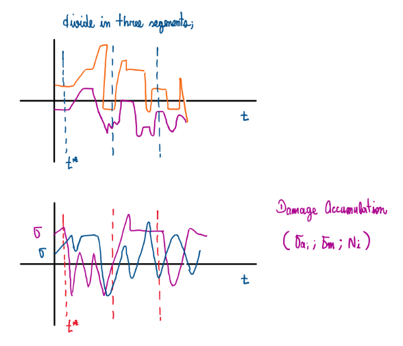
The load-time history is taken and divided in segments. Figure 22 indicates three common sections which can be evaluated. Inside each of them there are a sigma_a, sigma_m and ni for these cases. In addition it is also possible to compute Ni.

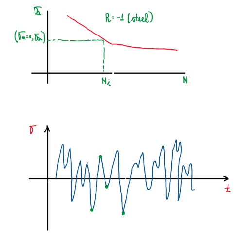
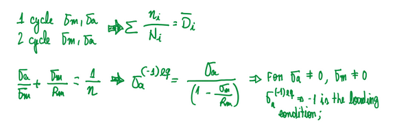
For each segment it is possible to build a S-N graph and with ni and N_i it is possible to calculate the damage accumulation (Figure 23). The Haigh equation separates the oscillate part from the constant part of the signal. R equals to -1 is the loading condition, thus the equivalent local stress can be calculated:

Hence, the summary of this approach is:

1. Select a significant story;
2. Perform the cycle counting;
3. Sigma_a; Sigma_m and ni;
4. Calculate damage using mean stress effect;
5. Determine the repetitions.

The value obtained from D for practical application is usually in the range of 0.1 and 0.3. The meaning of this number is similar to the safety factor, with the difference that it is possible obtain this data converted from cycles to a unit which has meaning for who is analyzing. For instance, in the racing field, it is possible to calculate the damage accumulation converting the number of cycles in mileage, laps or even races. This is quite important since the number of cycles has no meaning in the field.

References

1. Norton, Robert. Machinery Design, McGran Hill, 4th Edition;
2. McKelvey S. A. Yung–Li L. Barkley, M. E. Stress-Based Uniaxial Fatigue Analysis Using Methods Described in FKM-Guideline. J. Fail. Anal. and Preven., 12, 445-484, 2012;
3. Pedersen, M. M. Introduction to Metal Fatigue. Aarhus University, 91, 2018, ISSN: 2245-4594.