The procedure to evaluate the fatigue life in components for racing cars usually is based on three main sources of information, regulations, performance target and track the data. This can vary according to the company culture, but usually the g-g diagram is the main data provided by the data acquisition systems. Driving simulators and finite element analysis (FEA) are also used as tools to evaluate the fatigue life of a component. The main objective of the fatigue life calculation is to avoid a failure during a race and an outing. In addition, it also helps reduce parts weight and cost. The procedure can follow three steps:

• Calculate the fatigue cycle using all the fatigue loads;
• Calculate the fatigue cycle using all or 95% of the track loads;
• Calculate the fatigue cycle using the simulation data.

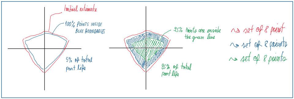
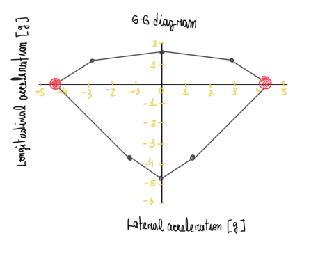
The g-g diagram is built using the information from the vehicle dynamics department and real data from acquisition systems, as Cosworth and Motec. The first is used to define an initial estimate of the vehicle performance, usually mentioned as what it should be. Hence the real data is plotted on the same diagram. The difference between “what it should be” and “ what really is” should not be big, because this means that the real car either is to heavy or too slow. After defined the g-g diagram, the plot of the real data is subdivided in 2 or 3 groups. These are the one of dots that should be inside the initial estimate boundary. The population are usually defined by the percentage of information used, thus P100, P95, P50 and P0, which means 100, 95, 50 and 0 percent of the track loads. It is important to mention that these one do not account the misuse loads. Although there are many dots on the diagram and each of them represents a vehicle maneuver, only nine of these are really important in the evaluation of the fatigue:

• Kerbs;
• Pure braking;
• Combined braking cornering outer wheel;
• Pure cornering outer;
• Combined acceleration cornering outer wheel;
• Pure acceleration;
• Combined braking cornering inner wheel;
• Pure cornering inner;
• Combined acceleration cornering inner wheel.

However, the fatigue calculation does not consider all the events faced by the car, instead, only critical ones. This is called conservative approach, because the vehicle is not exposed to this forcing level all the time. In fact, one cycle occurs when all the loads above mentioned are applied in the sequence which was listed. This is applied to the lap distance. A lap is usually evaluated by time, but in this case it is considered the distance. Hence it must correlated the distance (km) with the cycles, which 1.5 cycle per 1 km. In other words, the loads listed above in sequence repeat 1.5x in 1 km. Fatigue calculations are based on cycles of initial statements, 100 or 95 percent of the track loads (Figure 2). Once the cycle is established, the forcing are introduced and failure mileage is calculated. Obviously that as the loads are higher, the mileage became lower. The results, actually suggests if it is safer to go thinner and lighter with cross-section of the components, which is the main objective in the racing field. After defined the component, the mileage informed in the manuals are always lower than the component is really able to hold. This helps to keep the customers under control relative to the maintenance intervals of these components.

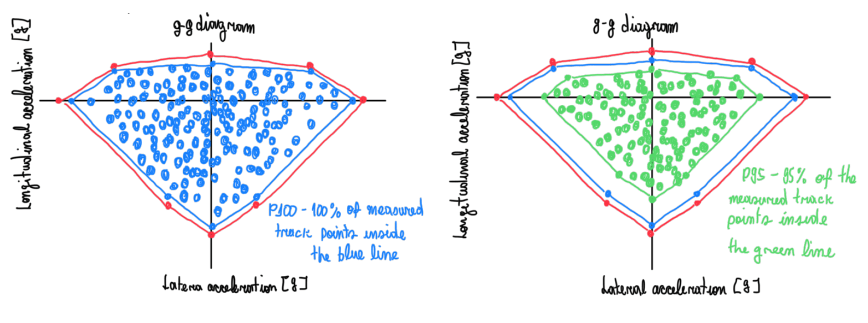
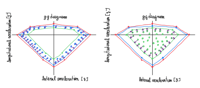
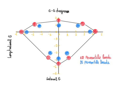
As seen in Figures 2 and 3, after defined the lines for the initial estimate (red one), 100% (blue one) and 95% (green one), the populations between P100 and P95 are transposed to the P100 boundary, these will be the representative of the 5% of the total part life. The populations from P95 until P0 are transposed to the P95 boundary. Hence this case represents the life cycle of 95% of the total part life submitted to the track loads. For instance, if the part considered should operate for 30,000 km, thus the amount of cycles will be 45,000. In addition, the P100 will represent only 1500 km or 2250 cycles while P95, 28500 km or 42750 cycles.

This approach can vary according to car companies, for instance, there are cases which eight points are taken into account, as can be seen in Figure 4.

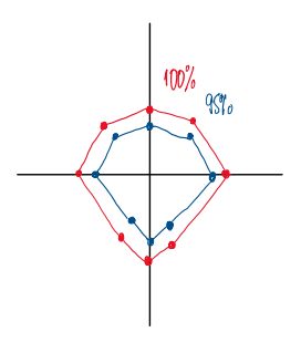
These eight point are respective to the most critical points that a race car must afford. Therefore the entire population under these boundaries are reduced to these points and submitted to 1.5 cycles per 1 km. This can be calculated by the tire revolution which is converted in km. In addition, with the knowledge of the track path, it is possible to evaluate how much the car is requested in each track sectors.

Wheel hub fatigue calculation procedure

The wheel hub is a rotating component, thus its fatigue calculation has some different steps relative to components as wishbones and uprights. Basically, the method follow three consecutive approaches:

1) Usual approach;
2) Discretions track replay;
3) Full spectrum track replay.

Usual approach

Basically is the same approach performed for the wishbone, the vehicle department is the source of the track or simulator data. However, the fatigue calculation is conducted only for the highest reached load of the car. Hence, it is assumed that the damage is accumulated by the pure cornering situation, which is when the vehicle is near the cornering apex and without any longitudinal acceleration, all the tire potential are being used for cornering. In addition, it is considered the outer wheel. As applied for wishbones, the cycle is repeated 1.5 times every kilometer. However, for wheel hub the cycle is composed by pure cornering outer wheel at 0 ̊ and 180 ̊. In other words, the load which the
outer wheel is submitted when the car is in a left side corner and then take a right side one. The loads considered are the 100% of the design loads, which are the one defined in the project requirements by the vehicle dynamics department. These represents the maximum achievable car performance.

Discretized track replay

This approach is an extension of the previous one which only assumed pure cornering. Since this is just one of the many maneuver that a race car usually perform at a race track, the others are simplified in representative maneuvers.

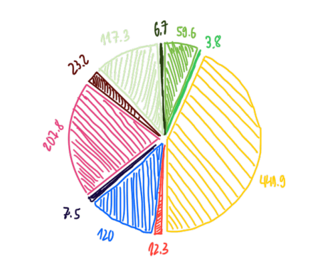
The vehicle dynamics department usually give the mileage that of the race car (Figure 7). This is the data about the elapsed mileage in each loading. For example, Figure 7 illustrates that the vehicle runs just 7.5 km at pure cornering outer of 100% of the design loads. However, it runs 120 km at 95% of the design loads. The values illustrated above were normalized by a distance of 1000 km. Hence, for 1000 km, this
car run 120 km at 95% pure cornering outer load. As can be noticed, there are data at 100% and 95% design loads, these are called high and low, respectively. Since there are many loads which a race car is exposed in a lap and is already known that the pure cornering is one of the highest, the other loads are simplified between pure cornering, pure braking and pure acceleration by intermediate maneuvers. These are also given at high and low conditions.

At this case the routine of analysis seen in Figure 8 can be summarized below:

• Pure cornering low 0 ̊;
• Pure cornering low 180 ̊;
• Pure cornering high 0 ̊;
• Pure cornering high 180 ̊;
• Maneuver low 0 ̊;
• Maneuver low 180 ̊;
• Maneuver high 0 ̊;
• Maneuver high 180 ̊.

This cycle also repeats 1.5 time per kilometer. A simplified version of this approach is the one which consides the pure cornering maneuver only, but with more percentiles of the design loads.

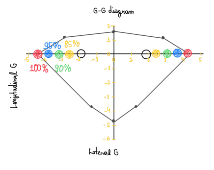
Figure 9 illustrates that 100, 95, 90 and any specificied percentile of the design loads are considered and the fatigue is accumulated for each of these cases. Hence, the routine of the damage accumulated due to fatigue is:

Fatigue cycle at 100% loads for n₁₀₀ cycles
Pure cornering outer/inner at 100% and 0 ̊;
Pure cornering outer/inner at 100% and 180 ̊;
+
Fatigue cycle at 95% load for n₉₅ cycles
Pure cornering outer/inner at 95% and 0 ̊;
Pure cornering outer/inner at 95% and 180 ̊;
+
Fatigue cycle at 90% load for n90 cycles
Pure cornering outer/inner at 90% and 0 ̊;
Pure cornering outer/inner at 90% and 180 ̊;
+
Fatigue cycle at x% load for n_x cycles
Pure cornering outer/inner at x% and 0 ̊;
Pure cornering outer/inner at x% and 180 ̊;

The last percentile is defined according to the design requirements and application, usually is an specific percentile to evaluate an specific load or situation.

Full spectrum track replay

This approach consider again the pure cornering maneuver, but using real lateral acceleration data from the car which is applied directly into the wheel hub. Hence it is considered the pure cornering outer for left and right side corner, 180 ̊ and 0 ̊, respectively. Therefore, a FEA is feed with these data to perform the fatigue simulation.

Comments for wishbone fatigue analysis

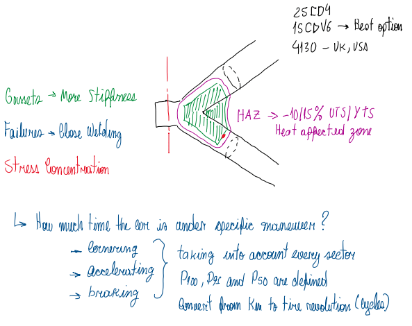
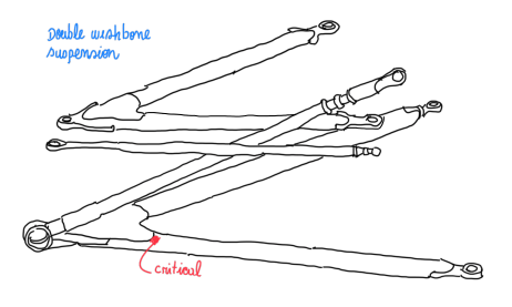
Considering two tubes that should be connected to form the wishbone suspension arm. The junction is made by welding of a part called gasset (Figure 10). This profile has the function of hold together the two tubes and improve the stiffness of the wishbone at that region. This is done because welding is a common source of failures. Since wishbones suffer some buckling and the regions at that point of the wishbone are exposed to high temperatures due to the brake system, thus they are heated affected zone (HAZ). Just an HAZ is capable to reduce UTS and YTS about 10/15%. The main materials used for the tubes are steel alloys 25CD4, 15CDV6 and 4130.

Nowadays race car companies have a lot of resources rise data about a future vehicle which is in design process. For instace, the driving simulators can provide data which very near to the reality. However this method still is somewhat conservative, since the track laps are not always the maximum of the vehicle performance. Hence, this approach is, in some degrees, similar to the one described in the previous paragraphs, using the G-G diagram.

References

• This article is basically my understanding about one of the Chassi and Body Design lectures taught by Luca Pignacca and Gianni Nicoletto.