After extraction of the information in the data analysis system, the next steps is to take wheel load curves over time and makes a stress-time curve. This article will review the steps of the fatigue calculation in race car components, since the number of cycles neither the amplitude of the stress are not clear.

The loading condition during a lap are defined according to the following parameters:

• Maneuver;
• Specific point of the track;
• Wheel loads;
• Part forces.

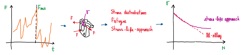
An important detail relative to these stresses is either they are at plastic or elastic deformation zones (Figure 1). Although the analysis is usually taken by similar methods, it is important to define what are the main informations. In addition, the conditions also defines which approach to choose.

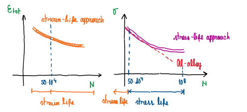
In general, the strain and the stress life approaches are used for low and high cycle load cases (Figure 2). The automotive industry commonly uses the stress life approach. However, these designations are not restrictive. It is interesting to understand what and which information the engineer wants to extract from the calculation.

Hence, there are situations which the plastic behavior of the material define the kind of approach adopted. In general, misuse loads are always taken into consideration with the strain life approach, because it is important to identify the material behavior when the material reach the plastic condition.

This method helps to define the effects of microcracks, but for this one, the designer usually assumes that there are micro cracks in the material (Figure 4). This is not the approach used in the automotive field. In general it is common in the aerospace industry. The microcracks always propagate to macrocracks. The automotive design assumes that the material does not have microcracks. In any case, there are some techniques used to avoid microcracks. The shoot peening and the rolling are the most used ones.

The shoot peening performs a plastic deformation on the surface to create a layer with a very high stressed material which covers the softer one (Figure 5).

As bolts are components which are very exposed to stress concentration, thus the shot peening can be done. Actually, the process name is rolling, which most stressed zones are plastically deformed by rollers. They create a fillet in those regions which also improves the surface appearance. To estimate the amount of residual stress developed after the rolling it is performed the x-ray refraction method (Figure 7).

It is possible to design a part with a smaller diameter, thus lightweight, but able to reach the same fatigue stress of 500 Mpa and at a high number of cycles. The idea is to adopt a test with a proper spectrum, which approximates as much as possible to the real part operating conditions. In this way, it is possible to find the maximum stress and cycles which a part can afford, thus using this method to explore very lightweight parts.

Stress life approach

This method assumes that the material is always at the elastic behavior. In this case, the fatigue estimation is exhibited by the so called S-N curve. Hence, the key parameter is the stress. It usually ranges from 50E+4 cycles to above.

Strain life approach

The main difference relative to the stress life approach is that it is based in cases which the components enter in a plastic deformation region. In addition, it is usually described for conditions below 50E+4 cycles. This limits the application of this method for specific cases. However, it is also adopted for components which a plastic deformation is induced on purpose. Hence, the strain life approach makes able to verify if the component is under its strain and stress limit.

Fatigue mechanism

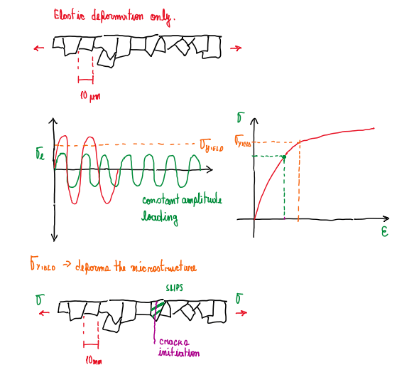
As can be noticed, a constant amplitude loading is a conservative approach to estimate stress and fatigue life. Once the material stress-strain curve is known, it is possible to evaluate how near or far from the yield stress the component are. Although a precise loading must be defined, this information can help the engineer to understand how tolerant the part is against a misuse. Hence, misuse loads are frequently introduced at the fatigue tests. At the microstructure point of view, the stress applied on a component deforms the crystal lattice of the material. In this way, at the stress level there are planes which this deformation changes them in the load and stress direction, in other words, it strains. However, at same time a portion of this deformation remains on the elastic condition. Hence, when the load is reduced, the deformation is completely reajoint. This is associated to the well known fatigue limit or very long life. However, this occurs only when the component is kept under elastic condition. When the load reaches a stress characterizing the material yielding, the microstructure suffer a plastic deformation. This distort the microstructure, so it changes its shape. The grain distorts by a mechanism called slip, which is a kind of plastic deformation. After returned to the no stress condition, this microstructure holds the distortion, but some portion are still in the elastic condition. The result is a crack initiation. For this reason, it is important to evaluate under the strain life method, because it is possible to estimate how tolerant the material is against misuse loads. The fatigue mechanism is a cumulative penalty, even the loads which are under the elastic deformation level may cause some microstructure portions to suffer a plastic deformation. Inside this some grains are displaced in a favorable direction, thus microcracks arise. These evolve during the cycles and became macrocracks. This is called crack initiation. Due to the unpredictability of grains orientation and elastic-plastic condition, the crack initiation is a statistical phenomena. The fatigue often occurs at the surface of the components, because the most mechanical cases have the most critical point at the surface due to several reasons. Some of these are that the stresses are higher at the surface (Bending, shear and torsion), the variation of the cross-section and the effects of the environment. Hence the plane of the crystalline structure and its grains slip during loadings. The slip goes through grains which became plastically distorted. However these performs monolithic plastic deformation which can not be observed with visual analysis. As the load continues, more and more slips are occurring and new grains became plastically deformed. The ones which already were plastically deformed are more stressed. Some of them are in the limit of material yielding, and then crack. The component does not exhibit any operational effect and the fracture occurs without advice.

Fatigue strength improvements

As developed in the previous topics, fatigue strength is basically a superficial failure which progressively propagates through the material microstructure. Hence a possible solution would be the application of a stiffer material. As a result, the component became brittle and, in most of the cases, heavy. There are some technological features which can improve the superficial stiffness of the components. The objective is to plastically deform the part surface which creates a layer of stiffer microstructure. There are two main procedures used to perform this modification, shot peening and rolling.

Shot peening

The shot peening is a process which many metal spheres are shot against a component. It is widely used in components as gears, crankshafts, springs, rods and bolts. When applied to parts made by high strength steel (HSS), the process can generate compressive stresses up to 55% of the ultimate tensile strength (UTS). One common example is a machine bolt or the assembling bolt, washer and nut. These usually have a smooth section of the thread, which is called shank. When the bolt is under axial stress, each screw of the thread is exposed to the components of the axial load. The critical thread is the first one, because the other screws are exposed to smaller portions of the axial load. Hence this may be the most critical point in a bolt. In fact, bolts usually have some points which are candidates to be the most stressed ones. These are between the head and the shank, on the first thread or the first thread under stress. This last one usually easy overcome the stress which the bolt head is exposed. In fact, this part might became critical at the moment of the fastening torque. To avoid this condition shot peening is successfully applied, which improve the yield strength and also provides an aesthetically better surface. However, for the thread part, the process is different. In fact, it is more related to the bolt manufacturing process than to a post process.

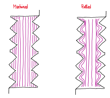
Usually bolts are made by machining or rolling (Figure 8). Basically, in the first case the material is cut and there is no or small amount of residual stresses. The other option is rolling. An ingot is forced against a screwed hole and get out of it threaded. This process implies a plastic deformation of the material surface, thus a residual stress made due to the compressive loads which plastically shape the thread. The result is a more strong threaded shank. Since there are several option and manners to improve the residual stresses, the same can not be said by the estimation of how much residual stresses was applied to the material. In fact, it is difficult, because this effect occurs due to the microstructure modification. The method used is the x-ray refraction. The lattice deformation can be detected and evaluated by the ifference between the angle which the ray reaches the structure and its angle after refraction (Figure 7). This occurs because the distance between fibers change or reduces when a plastic deformation is imposed to the material. In this way, it is possible to estimate the amount of residual stress. This is important for parts and components which operates with a pre-load.

Fatigue analysis

The fatigue resistance of a component is not a straight-forward calculation. There are a lot parameter which influence on the result, these can
have a great or a smaller impact. For this reason the methods of fatigue analysis and the information used on it are very important. Usually, the first step is the complete understanding of which design load will be adopted. It can be the maximum or the minimum load. If the first is used, the result would be too conservative, which means excessively heavy. On the opposite case, the result would be too weak for the application. Hence this decision should take into account some information about the system and this is the starting point. In the race field there many sources of information. As soon this is already defined, there are some softwares that helps to improve and to understand their meaning, the N-Code is one of these.

Figure 9 illustrate the use of the loads registered in track test and used to evaluate the fatigue analysis of the component. In the big screen it is possible to visualize some graphs. The strain-time is the main one, it is used to build the spectra of the loading condition. In other words, the number of cycles at which the strain values are occurring. In fact, the spectrum of a loading is not well defined for all cases. There many kinds of spectra for applications that goes from automotive to aerospatial. For instance:

This is a common spectrum used in the aerospace field (Figure 10). The load sequence is based in steps, each of them has its own stress value and the thickness of the block represents how much cycles at that respective load the step longs. It is a process of 15 steps that repeats itself after the step 8. This is the longest one and with the highest load. After this, the spectrum graph can be performed which exhibits the cumulative frequency distribution, also in function of the number of cycles, L_s.

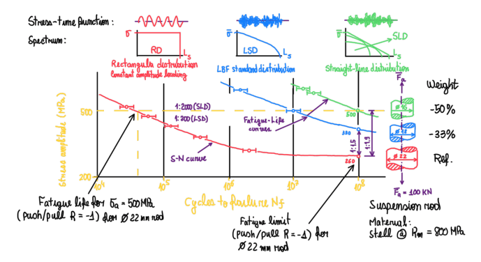
Figure 11 there three kinds of suspension rods being evaluated, they have 22 mm, 18 mm and 16 mm diameter and are exposed topush/pull test of 100 kN. The first situation, 22 mm diameter rod, results in a fatigue limit of 260 Mpa at E8 cycles. This is a long-life component for sure. However, if it is considered that this rod is exposed to 500 Mpa stress which is a result of a rectangular distribution RD. As can be seen, this loading configuration results in a progressive reduction of the fatigue limit of the rod. However, if another test is done with 18 mm rod using other distribution, it is possible to have a fatigue limit of 500 Mpa, but at higher number of cycles. In fact, what Figure 11 illustrates is that the kind of loading has a great influence on how high can be the fatigue limit. The LBF standard distribution is a kind of loading developed in Germany by LBF institution. Finally, the last case is the 16 mm rod which is exposed to the loading distribution SLD, straight line distribution. It reaches 500 Mpa at highest number of cycles of all cases. Therefore, Figure 11 suggests that with the proper information and evaluating carefully its spectrum, it is possible to choose the loading distribution that best fits situation, or to build a loading distribution that emulates the real conditions. Driving simulators can help a lot in these cases together with track test data. Hence, with correct spectrum and load distribution for the loading condition, it is possible approximate to a lightweight construction with a controlled loss of durability.

Rain flow approach

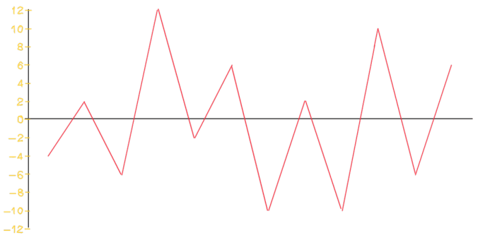
How to determine the amount of cycles present in this piece of loading history at Figure 12? In fact, with a constant load case, the mean stress can be give by:

However for the case in Figure 12 which is not possible estimate the amplitude, it is applied the rain flow approach, or counting cycles approach.

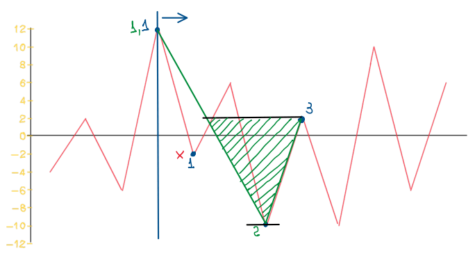
The procedure to combine the stress level at different points of the stress history. For instance, at Figure 14 it were established three stress levels, 1, 2 and 3. Considering the stress level 1 at the first peak, the next stress level is too small compared with the first. In theses cases it is not possible to consider that they form a cycle, because the first stress level has a modulus much higher than the next one. Hence, this is neglected and the stress level 2 is highlighted in by the green line. In this case, the stress level 2 together with the first stress level one can be considered a cycle.

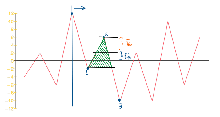
It is also possible to consider another stress levels (Figure 15). In this case case, from the stress level 1 to 2 it is possible to see that the first has a stress range lower than the second stress range which can be written by (Figure 16):

The same rule can be applied for this first example. Therefore, the rainflow rule can be defined as:

Basically, the rain flow approach is based in two stress deltas taken between three points over the stress history. If the first delta is lower or equal to the second delta, these three points can be assumed as cycle (Figure 17). It is important to remember that the rainflow technique is based in the spectrum chosen to represent the loading of the situation under analysis. For this reason, the correct choosen of the spectrum is so important in the fatigue analysis.

References

1. Norton, Robert. Machinery Design, McGran Hill, 4th Edition;
2. McKelvey S. A. Yung–Li L. Barkley, M. E. Stress-Based Uniaxial Fatigue Analysis Using Methods Described in FKM-Guideline. J. Fail. Anal. and Preven., 12, 445-484, 2012;
3. Pedersen, M. M. Introduction to Metal Fatigue. Aarhus University, 91, 2018, ISSN: 2245-4594.