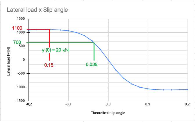
The tire modeling by the Paceijka model allows to perform fast calculations about the tire performance. In the absense of a tire data it is not possible to evaluate a the tire performance. However, with just one graph it is possible to estimate the behavior of this tire. Hence, considering Figure 1 which illustrates the plot of the lateral load F_y per theoretical slip angle. The objective is to find the coefficient of the Magic formula which is given below. This article will perform some calculations using graphs as the only information available. The method applied can be easily used in the field to retrive fast and qualitatively good informations about the tire performance.

y = Dsin[Carctan{Bx-E(Bx-arctan(Bx))}]

The method is based in guesses, thus as experienced the profissional is, near the real case the tentative will be. The first parameter to be estimated is the vertical load F_z. A good guess for this case is 700 N or 0.7 kN and this will be the first try. Later 550 and 200 N will also be estimated. Since F_z is estimated, it is possible to guess the parameter D when the tire is under the peak of F_y which by Figure 2 a good tentative is 1100 N. Hence, by the equation of D it is possible to calculate the friction coefficient:

D = y_m = μ*F_z

μ = y_m / F_z = 1100 / 700 = 1.57

The next step is to guess the assymptotic value y_a, which represents the lateral load produced at very high slip angles. This is a condition which the tire already reached the maximum performance, but the slip angles continues to increase. Usually, F_y decreses until reaches a almost constant force, which is dramatically lower than peak F_y. A good guess is 800 N and the following equations can be applied:

y_a = lim_x→∞ y(x) = D*sin(C*π/2)

C = 2 – (2/π)*arcsin(y_a/D) = 2 – (2/π)*arcsin(800/1100) = 1.48

D and C are already found, it lacks B and E which are correlated with the cornering stiffness. By the definition, this is given by the derivative of the lateral load by the slip angles. However, after the linear portion of the curve finishes, the cornering stiffness (Figure 2) decreases until reach zero, which is the condition for the peak of the lateral load, F_y. The cornering stiffness is given by y'(0) and should be estimated to allow the calculation of the parameter by the following equation:

B = y'(0)/(C*D)

Using Figure 2 to guess y'(0) it is possible to find 20000 N/rad, thus applying in the equation above:

B = 20000/(1.48×1100) = 12.28

The parameter E depends on B and x_m, this is the slip angle at the peak of Fy, thus it can be estimated by Figure which suggests that xm is equal to 0.15 rad. Hence, the following equation can be applied:

B×(1 – E)×x_m + E×arctan(B×x_m) = tan(π/(2C))

E = [B×x_m – tan(π/(2C))] / [B×x_m – arctan(B×x_m)] = [12.28×0.15 – tan(π/(2×1.48)] / [12.28×0.15 – arctan(12.28×0.15)] = 0.07

Now, with Fz, μ, B, C, D, and E, it is possible to visualize the curve fixing these parameter, which were found by estimation and guessing, and applying the slip angles seen in Figure 2, which goes through – 0.2 to 0.2. Hence, for Fz, μ, B, C, D, and E which are equal to 700 N, 1.57, 12.28, 1.48, 1100 and 0.07, respectively, the estimated curve can be compared to the original one.

As can be seen on Figure 3, basically the guessed plot superposes the original one, which means that the results were approximately the same. It is possible to verify also the values from the original curve as suggested by Figure 4.

The values are almost the same. The guess of the y_m (1100 N) almost reached the real value, which is 1099.2 N. In addition, the value obtained from estimations and application of the magic formula was 1099.162 N, basically the same value.

Assymptotic value sensitivity

Since the estimations and calculations were well succeeded, now it will be evaluated the asymptotic value ya variation and its influence on the plot.

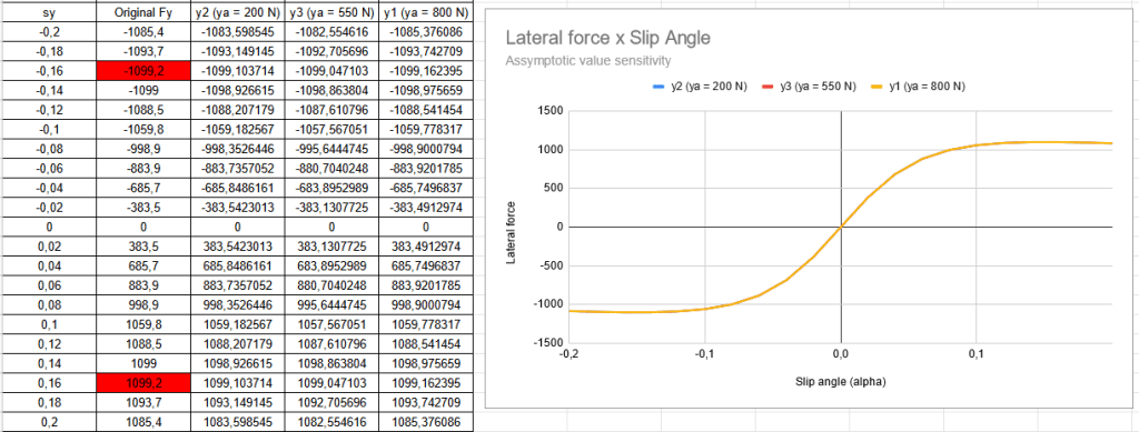
In fact, y_a is a condition which the tire is being operated out of its boundaries. In this situation the friction coefficient changes to the kinetic value. The result is a dramatic reduction of the lateral load. If the tire is kept at this condition, the lateral force reach its lowest value and then, became constant. In the Paceijka model this is callled assymptotic value. Figure 5 illustrates three iterations with different y_a, 200, 550 and the first one, 800 N. The interesting point with these iterations is that after plotting the curves, they are practically superimposed. This suggests that the sensitivity of the magic formula to the assymptotic value y_a is very low. Hence, it is suggested to start the iteractions by y_a, because after defined it, C can be found by the following equation:

C = 2 – (2/π)×arcsen(y_a/D)

Hence, B and E can be defined. Even if y_a drastically varies, the other coefficients are weakly correlated to it. A good guess for y_a lies in the range of:

0.2 < y_a/y_m < 0.85 => y_a/y_m = 800/1100 = 0.73

Therefore, the guess made it in the firsts paragraphs are inside this range, thus feasible to deliver good results.

Vertical load sensitivity

The first step in the analysis of the vertical load F_z sensitivity on the lateral load F_y is account its influence on friction coefficient µ. Hence the following equation is introduced:

µ = µ₁ + (k×F_z)

Where µ is the friction coefficient obtained by D equation in the beginning of the article, µ₁ is the friction coefficient resultant due to Fz, k is a derivaritive coefficient, given by k = dµ/dF_z. In the calculations performed in this article, k is equal to -0.05 kN^-1. Hence, it is possible to calculate and plot the the impact of F_z in µ₁.

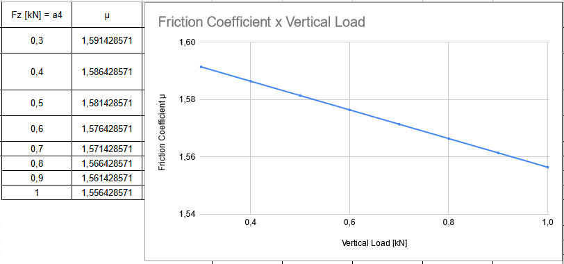
Figure 6 illustrates the effect of Fz, a progressive decrease of the friction coefficient µ1. This suggests that as more vertical load is over the tire, less capability to produce grip it will have. Hence, the friction coefficient equation is now added to the D equation:

D = µ×F_z = [µ₁+(k×F_z)]×F_z = [a₂+(a₁×F_z)]×F_z

As can be seen, to account F_z sensitivity into the magic formula, the parameter D is now in funcion of two new parameter, a₁ and a₂ which are k and µ₁. Hence, B, C and E now have more coefficients inside their equations which are summarized below:

B×C×D = y'(0) = a₃×sin(2×arctan(F_z/a₄))

B = B(F_z) = y'(0) / (C×D(F_z)) = (a₃×sin(2×arctan(F_z/a₄)) / (C×Fz×(a₁×F_z+a₂))

C = 2 – (2/π)×arcsin(y_a/D) = a₀

Where a₁, a₂, a₃ and a₄ refers to k, µ₁, y'(0) and F_z, respectively. In addition, there is another coefficient named a₀, which refers to the parameter C. With these equations it is possible to build the Magic Formula in function of x, which it refers to the slip angle and y refers to the lateral load.

Figure 7 illustrates that increasing the slip angle, which is given by the theoretical value σ_y, the lateral load F_y also increases. However, if σ_y is fixed, for instance at 0.05, it is possible to verify that the increase of the vertical load F_z allows to the tire produce a higher F_y with the same σ_y. This is a quite important conclusion, but it does not means that increasing the vehicle mass generates a better grip. The reason is the reduction of µ seen in Figure 6. This is also valid for the lateral load transfers. However, if the vertical load considered is due to the aerodynamics, this is quite useful, because Fy increases without the penalization seen in Figure 6. The aeroload is weightless load.

Another interesting graph is seen in Figure 8, which illustrates the plot between the cornering stiffness and F_z. By this one it is possible to visualize the parameters a₃ and a₄. These are the cornering stiffness at the peak y'(0) for the reference vertical load considered, respectively. The reference F_z for the example analyzed in this article is 700 N or 0.7 kN, which according to Figure 1 produces y'(0) of 20000 N/rad or 20 kN/rad. Hence, Figure 8 illustrates why a₃ and a₄ are 20 kN/rad and 0.7 kN, respectively. However, Figure 7 hides an important information. Since it was already explained why the grip produced as Fz increases, this should be seen in Figure 7, but if the lateral load Fy is evaluted normalized by Fz, the graph explains more why at some point the Fz increasing does not represent better grip.

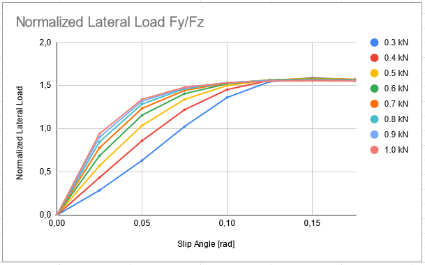
Figure 9 illustrates that as F_z increases, F_y also increases, but not in a proportionally relative to F_z. Actually, F_y increases less and less until a threshold which there is no more gain. As already mentioned in the previous paragraphs, occurs due to the µ penalization relative to F_z. Hence, as more F_z, more F_y, but at a cost of µ reduction. At some point this will be higher than F_y gain, as seen in Figure 9 in the curver of Fz equals 0.9 an 1.0 kN.

Lateral load transfer

Once Fz sensitivity is verified, it is possible to evaluate the lateral load transfer effects in the axle. Actually, the graph for this case also helps to understand the Fz sensitivity. It is important to understand that this is not totally intuitive. Hence, considering a situation which 0.1 kN of vertical load Fz is transfered for one wheel to another from the same axle and take advantage from the previous calculations, Figure 10 can be produced.

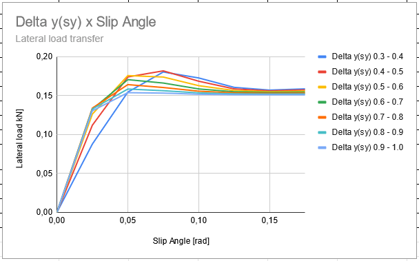
As can be seen, at low slip angles almost all cases has the same behavior, the curves basically are superimposed with exception by the curves red and blue. It is also possible to visualize that the highest Fy is produced about 0.75 rad. Figure 10 suggests that lateral load transfer under high vertical loads produce lower Fy. However, at these cases, the peak of Fy cames at lower slip angles.

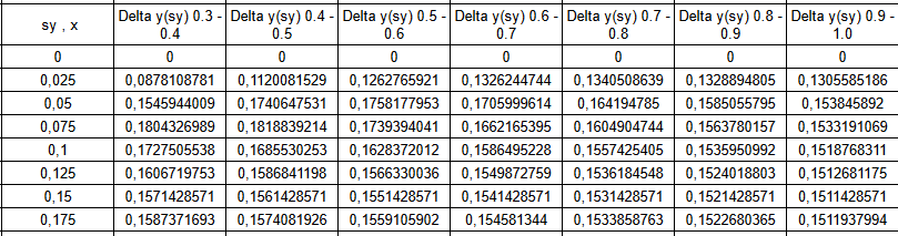
Figure 11 illustrates the table from the values calculated to plot the graph on Figure 10, it is possible to confirm that for lower Fz, the Fy generated is higher, but at high slip angles, 0.075 rad while for higher Fz the slip angle for the peak of Fy cames at 0.05 rad. If these values are normalized by their respectives Fz it is possible to plot the same curves which are in Figure 10, but now being the normalized lateral load transfer.

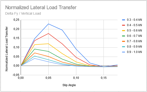
Figure 12 confirm that the excessive increase of F_z provide progressively less gain, that at some point there is a reduction. Hence, the vehicle capability to corner at very high speed is connected to the vertical load over the tires. This, if provided by the vehicle mass will penalize tires grip, but if it is provided by the aeroload, downforce, it allows the vehicle to run at very high speed through corners (medium and high speed ones). However, there is a hiden detail in Figure 12. The highest F_y are obtained at lower slip angles. This agrees with the fact that higher downforce results higher F_y at lower slip angles. Even though this is a great advantage, at some point a great downforce will result in too much low slip angles that disturbs the tire heating. Slip angles are necessary to heat the tires and produce grip, thus the grip can decrease even at very high F_z.

Pure lateral slip

The method previously adopted can be applied to any tire curve, Figure 13 illustrates the example. Now the reference Fz is given and parameter B,C, D, E, a0, a1, a2, a3 and a4 must be found.

Hence, the reference curve is the one respective to Fz = 4000 N, which are in the middle. Just with Figure 13 it is possible to estimate x_m, y_m, y'(0) and y_a, from these the other parameters can be calculated by the equations mentioned previously.

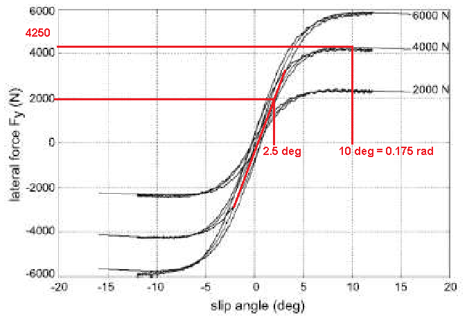
Figure 14 illustrates how it is possible to guess these parameter, thus the calculations are:

x_m = 10° = 0.175 rad

y'(0) = a₃ = 800 N/° = 45836.62 N/rad = 45.84 kN/rad

D = y_m = µ×F_z = 4250 ; µ = 4250 / 4000 = 1.063

µ = µ₁ + (k×F_z) ; µ₁ = µ – (k×Fz) = 1.063 – (-0.05×4000) = 1.263 ; a₂ = 1.063 ; a₁ = – 0.05 kN^-1

a4 = F_z = 4000 N = 4.0 kN

y_a = 3900 N = 3.9 kN (guessed)

These calculations are used as base to find B, C and E which are summarized in Figure 15:

Since in Figure 14 it is possible to guess ym, xm, y'(0) and ya, this parameter feed the following equations:

D(F_z) = y_m = (a₂ + (a₁×F_z))×F_z

B×C×D = y'(0) = a₃×sin(2×arctan(F_z/a₄))

B(F_z) = y'(0)/(C×D) = (a₃×sin(2×arctan(F_z/a₄)))/(C×F_z×((a₁×F_z)+a2))

C = 2 – (2/pi)×arcsin(y_a/D)

Therefore, it is possible to use as Fz reference 2000 and 6000 N to estimate the other two curves by the same method described above and plot the Magic Formula curve for each case as seen in Figure 16.

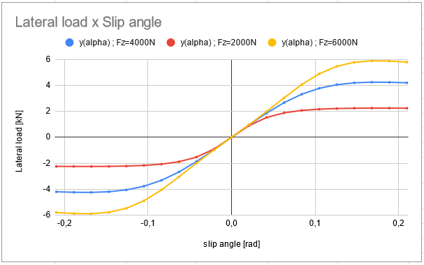
Hence, comparing the results on Figure 16 with the plots illustrated in Figure 14 it is possible to conclude that there is a good approximation. The only difference between Figures 14 and 16 is that the graph in this last one is exhibited with slip angles in radians for personal preference.

Pure longitudinal slip

All the examples given in the previous paragraphs refer to situation of lateral loads, but the magic formula can also be applied to longitudinal loads. Figure 17 illustrates a curve of pure longitudinal slip in braking case and the same method applied previously will be adopted here.

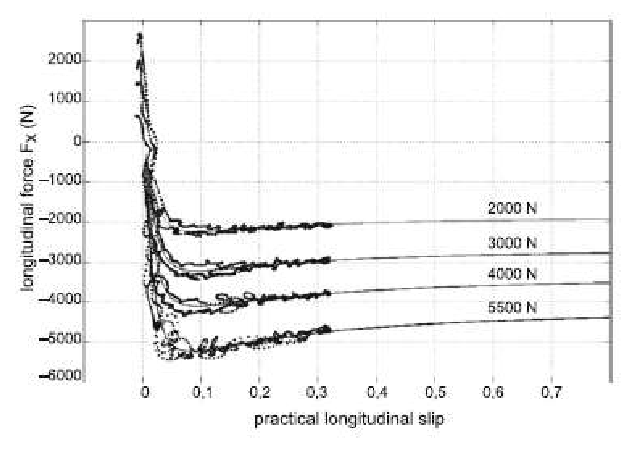
At this case the same conditions applied in the pure lateral slip will be adopted, thus reference Fz will be 4000 N or 4.0 kN. It is important to be advised that now the analysis will be performed relative to practical longitudinal slip σ_x.

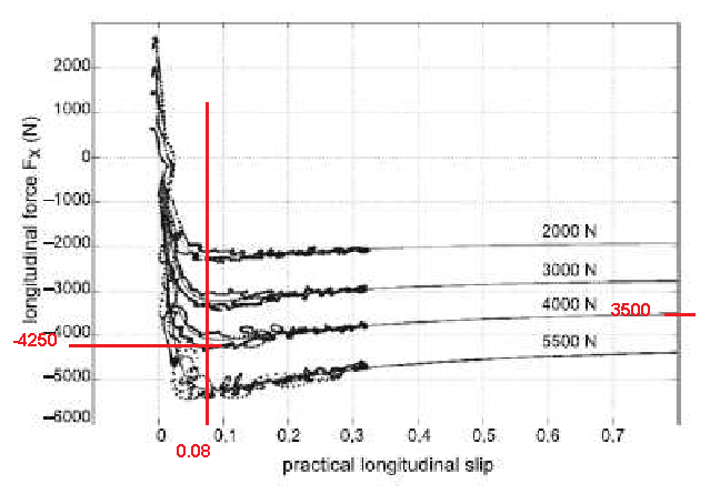
Figure 18 illustrates the points of the graph which it is possible to subtract the requested information, which are xm, ym, y'(0) and y_a, the longitudinal slip σ_x at the peak, the peak of longitudinal force F_x, the longitudinal stiffness and the assymptotic value.

y_m = -4250 N ; D = µ×F_z ; µ = -4250/4000 = 1.063

µ = µ₁ + (k×F_z) ; µ₁ = µ – (k×F_z) = 1.063 – (-0.05×4000) = 1.2625

x_m = 0.08 ; y_a = – 3500 N ; y_m = – 4250 N

a₁ = -0.05 kN^-1 ; a₂ = 1.2625 ; a₃ = -4250/0.08 = – 53125 N = – 53,125 kN ; a₄ = – 4000 N = – 4.0 kN

Hence, these parameters can be applied in the following equations:

D(F_z) = (a₂+(k×F_z))×F_z

C = 2 – (2/pi)×arcsen(y_a/D)

B×C×D = y'(0) = a₃×sen(2×arctan(F_z/a₄))

B(F_z) = y'(0)/(C×D) = (a₃×sen(2×arctan(F_z/a₄)))/(C×F_z×(a₂+(k×F_z)))

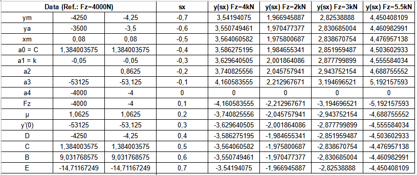
Figure 19 illustrates the calculations summarized in one table together with the calculatons of the Magic Formula. In addition, the same procedure applied for 4000 N reference vertical load was applied for 2000 N, 3000 N and 5500 N. The range of σ_x is applied accordingly of what was seen in the Figure 17.

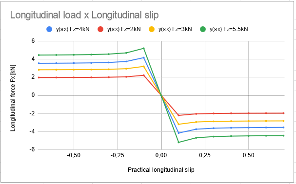
As can be seen, more F_z, higher F_x, better traction and grip. Another interesting point observed in Figure 20 is the highest stiffness y'(0) = a₃. If compared with the values from lateral slip (20 kN against 50 kN), it is possible to conclude that effects due to longitudinal load transfer are faster than the same for lateral load transfer. Figure 20 illustrates this by the high slope in the linear portion of the curve. In addition the assymptotic portion of the curve also appears sooner than in the lateral slip analysis.

References

• Race Car Vehicle Dynamics – Miliken & Miliken;
• Guiggiani, Massimo. The Science of Vehicle Dynamics. Handling, Braking, and Ride of Road and Race Cars. New York, Springer, 2014;
• Haney, Paul. The Racing & High-Performance Tire – Using the Tires to Tune for Grip & Balance. TV Motorsports, SAE, January, 2003.