The bicycle model of a car is one of the most commonly used model the vehicle dynamics. It is possible to make correlations with dynamic parameters of the vehicle relative to its tires, in other words, a bicycle model in function of the tire performance parameters. This article proposes a brief review about tire perfomance parameters their impact in the vehicle dynamics. In fact there are two main parameters, one based on the vehicle and the other based on tires, the side slip angle (ß) and the slip angles (α), respectively. These two are given by the following formulae:

α_f – α_r = ζ – ζ_ackerman → Understeer angle

β = (b/L) – α_r → Side slip angle

However, in the bicycle model there is another important parameter in function of the tires, the cornering stiffness. This is a ratio between the lateral force and the slip angle:

C_i = F_yi / α_i → Cornering stiffness

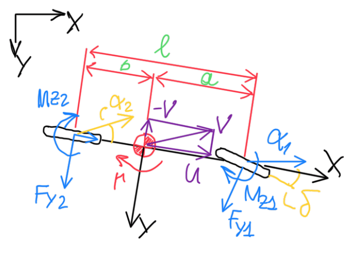
This is a quite interesting ratio, because it is called stiffness, but it has nothing relative to it. Hence this term is misleading. In fact, understanding it more deeper it is possible to have some conclusions about C_i. The unit is N/rad, because the slip angle α is given in radians. Hence the key point is α. Racing tires operates mainly by hysteresis. This parameter is extremely sensitive to speed. In tires there are many speeds, but it is no possible to evaluate the tire speed properly because of the tire contact patch compliance. Since the rim is the one component which is solid and stiff, there are two important speeds for tires, longitudinal and lateral speeds. The slip angle is ratio between the speed V and the fixed direction (Figure at the article cover). Since this speed has two components and α is ratio between two speeds, thus the cornering stiffness is basically the amount of lateral force for a specified speed. Therefore, C has nothing to do with stiffness or displacement, is a parameter more correlated to force and speed.

m∙(v̇ + u×r) = F_y1 + F_y2 → m∙(v̇ + u×r) + (C/u)∙v + (Cs/u)∙r = C₁∙ζ

I∙ṙ = a∙F_y1 – b∙F_y2 → m∙k²∙r + (c∙q²/u)∙r + (Cs/u)∙v = C₁∙a∙ζ

F_y1 = F_y1(α₁) ; F_y2 = F_y2(α₂) → Lateral force in function of slip angles

α₁ = ζ – (1/u)∙(v + a∙r) ; α₂ = – (1/u)∙(v – b∙r) → Slip angle at front (1) and rear (2)

Fyi = C_i∙α = C_Fαi∙α → Lateral force in function of slip angles and the cornering stiffness

From the slip angle, the understeer angle and the side slip angle equations, it is possible to find:

α₁ – α₂ = ζ – (l/R) = US → Understeer angle

Hence, from this point the main assumption of the bicycle model to analyze the tire performance and its effects is to consider a steady state movement. This is the neglection of the inertia. Since race cars are usually lightweight and their tire develop very high lateral and longitudinal forces, the inertial components can be neglected.

(l/R) = r/V ≈ r/u

a_y = V∙r = V²/R

α₁ = ζ = (l/R)∙[1 + η∙V²/(g∙l)] = l/R + η∙a_y/g

η = (F_z1/C1) – (F_z2/C2)

α₁ – α₂ = η∙a_y/g

η = – (mg/l) ∙ [(a∙C₁ – b∙C₂) / (C₁∙C₂)]

Therefore neglecting the inertial components, the transient loads are also neglected. This makes possible to assume that race cars operates quite often in a series of steady or stationary conditions, because most of their maneuvers are performed in steady or quasi-steady conditions. In some degree, this is a unique simplification for race cars, since road cars can not be designed without consider the transient loads. In this case, the range of operation is of low speeds, constant variations of acceleration and steering. In fact, road cars have a higher weight and a lower tire forces. Therefore, the transients in road cars is more critical with many inputs as acceleration, braking and steering.

Tire parameter

The main tire parameters which are important for vehicle dynamics are:

• Caster;
• Camber;
• Camber gain (with steering and symmetrical and asymmetrical wheel travel);
• Toe (Bump steer and roll steer with symmetrical and asymmetrical wheel travel);
• Scrub radius;
• Mechanical trail;
• Springs;
• Dampers.

These parameters have a great influence on the suspension kinematics and vehicle dynamics. The caster is the inclination of the line which starts from the top mount of the suspension and passes through the king pin seen from the side of the car (ZX plan) relative to the vertical. The caster influences on the steering response and usually is not the main adjustment parameter. In fact, the caster is first the set during assembling and it is barely changed after the car is ready to go. The camber is one of the main adjustment parameters, it defines the wheel inclination relative to the vertical but visualized by the front of the car, in other words, seen by the plane ZY. Hence, the camber gain is the variation of camber when the wheel follows a vertical displacement, even this one is symmetrical or asymmetrical. Any vertical displacement implies a camber variation. The toe is another important parameter, it describes the wheel inclination, but seen from above, or by the plan XY. This parameter also change with the vertical displacement of the tire, the so called bump steer or roll steer are variations of toe when the car bounces or turns. The scrub radius is the distance between the center of the contact patch and the king pin line extension until the ground. The assumption that tire forces are produced at the center of the contact patch requires the inclusion of a moment about the king pin axis. In fact, this is the torque around the steering axis. The tire force times the pneumatic trail (PT), which is the distance from the contact patch center to the king ping prolongation point is called self-aligning torque (SAT).

Torque around steering axis = SAT + F_y∙MT = F_y∙PT + F_y∙MT

As the contact patch changes, SAT is always changing according to the load applied over the tires. Hence, in some situations, what the driver is identifying as an understeering (loss of grip in the front wheels), can be only a variation in the pneumatic trail. Finally, the mechanical trail (MT) is the distance between the KPI prolongation point on the ground and the wheel center. The difference between these two trails is that mechanical trail, which fixed, because is defined by the suspension kinematics, but pneumatic trail changes almost constantly.

Tire working regions

The complexity of tires is the fact they operate in a very complex situation, the transition between linear and non-linear condition. In fact this is the region of the optimal performance of racing tires, but relative to road vehicle tires, these are operated at the linear zone. The reason is simple, it is safe and affordable, because tires which operates at the linear conditions are more predictable and cheaper to produce in terms of materials. The main graph that describes the tire performance is the lateral force by slip angle ones (F_y x α) that can be seen in Figure 3. In this one it is possible to visualize the distinct three zones of tire operation, these are called driving on grip, driving on slip and exceeding limit. The best way to understand it is drawing an iso-force line which describes that for the same force there is two different slip angles α. This occurs, because after the driver extrapolate the transition region (driving on slip), tires enter in a region which the force produced begins to fall. At some point, α produced are higher for a determined force, but this force could be produced at lower α without too much stress. This means that tires are not anymore slipping, instead they are suffering from slippage, which is a worst condition that produces more heat, more wear and less grip. In racing field, drivers are defined by their ability to work inside the transition zone, because this one is very easy to be exceeded or not reached. It is a very peculiar condition which the car controled slips over the track. Bottom line, fast drivers have the ability to manage the tire non-linearities.

Lateral force and aligning torque

The main tire force analyzed in race cars is the lateral force (F_y). This is usually correlated with the slip angle α. However, if in the same graph is put under evaluation F_y and SAT (which is also defined as M_z), it is possible to visualize interesting informations. There are two important points in Figure 4. First, at zero slip angle α, F_y and M_z are not zero. In fact, they null each other or the difference is too small for the driver notice some difference. The other point is the one at the peak of the lateral force. It is straight forward to observe that at this condition M_z almost zero. This suggest that, when the tire reach the peak of the tire performance in a turn, the driver starts to fell a different steering effort. In other words, the pneumatic trail is minimum, so SAT or M_z is low. At this condition what defines the steering effort is the lateral force. However, the driver is not able to distinguish between the lateral force (grip) and pneumatic trail. Therefore, what the driver feels, is the steering effort, M_z or SAT, but he/she is not able to differentiate between F_y or PT.

Pneumatic trail

The pneumatic trail is parameter which arises from the tire compliance. Hence the distance between the center of the contact patch and the king pin point times F_y is SAT. However the torque around the steering axis is given by the sum of SAT and F_y∙MT (mechanical trail). As already defined, pneumatic trail is minimum when the driver approaches the peak of F_y. Another characteristic of this situation is defined by the cornering stiffness. This parameter corretales the amount of F_y with the slip angle α developed. C is a tangent on the line in Figure 5. In the beginning of the graph, at zero α, C is almost constant. However it start to change as F_y and α increases further. In fact, C decreases as F_y and α increases. At some region of the graph, C is not linear anymore. This is called transitional range. If both are increased further, C reduces to to zero, thus the tangent is parallel to the horizontal line of the graph (Figure 5). The contact patch is working at two conditions, slip and slide. The linearity of Figure 5 (cornering stiffness) defines how much the tire contact patch is splitted between these conditions. In other words, the amount of area in slipping and sliding (Figure 6). At the linear conditions, racing tires are operating at almost full slipping conditions. At the opposite, when the tires is under non linear or C = 0 conditions, the contact patch is basically sliding over the surface. This is the desired condition by the driver and also the point which the best performance is extracted. It is important to mention that the cornering stiffness can not be evaluated by its linear definition (F_y/α). Instead, this parameter will be the local derivative of the tire at that respective situation, dF_y/dα. The key about the cornering stiffness is that there are two values for this parameter, the one for the front axle and the other for rear axle.

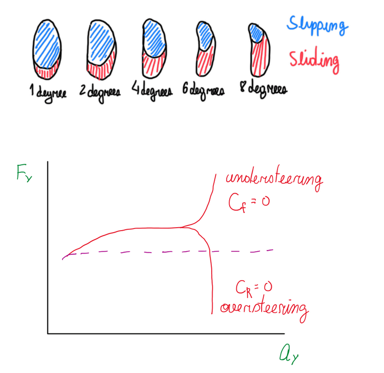
Hence, how fast one of these axle will reach the condition of zero cornering stiffness defines the vehicle behavior (Figure 6). In racing field, the engineers are not interested at linear local derivative situations, instead they want the car to approach the condition of null cornering stiffness according to the driver style and preferences. Hence, if C goes to zero at the front axle, F_y of front axle goes asymptotically to the negative infinite. Conversely, if the rear cornering stiffness goes to zero, F_y at ther rear axle goes asymptotically to the positive infinite. These are the regions of interest of the engineers relative to the tires.

Although the wheelbase is usually defined by L, the distance between the center of front and rear axles, it can change even though a bit during vehicle operation. This occurs due to the so called pneumatic trail. This is reaction of the tire rubber to the grip.

WB = a + b – PT_F + PT_R

Usually, the pneumatic trail is a rounded to the 1/6 of the contact patch length. Hence, it is possible to program this equation in data acquisition software and evaluate the wheelbase variation during vehicle operation.

Vertical load sensitivity

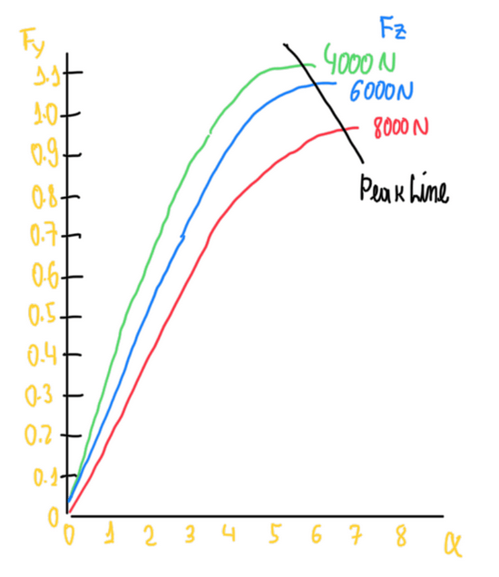
Tires increase their produced lateral force (F_y) by increasing the slip angle (α). However, F_y is a function of the vertical load (F_z) and the friction coefficient (μ). Even though F_y is proportional to F_z, the degree of proportionality is non-linear (Figure 8). Although the grip increases with F_z, as this became higher, the amount of grip available for cornering is lower. The result is a lower increment in F_y, thus a decrease of the lateral force coefficient. This occurs due to many reasons, the main ones are due to tire non-linearities, which can be represented by temperature, weight distribution, load transfer and friction. These also affects the tire contact patch which became non-linear, even though it also increases with F_z, not the entire area of it is under slip conditions. In fact, the maximum F_y is obtained at full slipping condition of the contact patch. If F_z increases further, the tire enters in the sliding condition and F_y drastically reduces.

Longitudinal forces

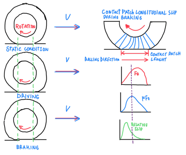
The contact patch also change due to forces. As can be seen on Figure 9, a tire when statically loaded, distributes the load over the contact area more uniformly. The friction produced is given by μ∙F_z. As the tire begins to rotate forward, the side walls suffers tension stresses which deform them towards the leading edge of the contact patch. The opposite occurs when the wheel is braked, the trailing edge of the contact patch is distorted. The peak of the friction force is obtained at certain amount of F_z. After this extrapolates a threshold, the friction reaches the dynamic condition and the friction force reduces. Therefore, the sidewall works applying proper forces to support the tire movement. In fact, tires must also deal with the different tension and compression on both sides (Figure 10).

There are some conclusions that can be made after these theories. The longitudinal forces are produced due to slip. It is required longitudinal slip to make the car accelerate. Since longitudinal acceleration results in longitudinal load transfer, the vertical load will vary. For this reason, the peak tire force also will vary together with the cornering stiffness. Bottom line, tires are devices sensible to slip and from this they creates grip.

Friction circle

The friction circle confirms (Figure 11) that the tire operation is all based at the development of the slip angles. First, the vehicle speed is an input. When the car is traveling and the driver steers, it is not only changing the steering angle, but also creating slip angle. This generates the grip that makes the car turn in.

As can be seen Figure 12, the correlation between the lateral force F_y and the brake force F_x depends of several parameters. Basically, α higher than 8°, makes tires to enter in the slide condition. Hence, F_y-F_x correlation depends mainly on α. However, the brake force alone is basically dependent of the longitudinal slip (k). Even though α results in its reduction, the brake force are higher at very small slip angles. In the opposite case, analyzing F_y alone, it only depends on α. However, as already seen by the friction circle (Figure 11), as the brake slip is increased, or the brake force, the lateral force drastically decreases. Tires operates under slip, but its friction is just one that should be distributed over the vehicle demand.

Tire drag

Figure 13 illustrates the coordinate system of a tire. As discussed previously, the deviation of the speed from the wheel centerline, which is where the tire is really pointing, creates the so called slip angle α. This is what generates the tire forces. In addition there is the drag. As can be seen, due to α, F_y deviates from the centripetal force and this creates a longitudinal component, but against the tire longitudinal movement which is called drag. The tire drag can be calculated by the following equations:

F_drag = F_y∙sen(α) = (m∙g∙G_y)∙sen(α)

However, a race car has another sources of drag and these, together with tire drag, consumes engine power. It is possible to account each one of these sources with their proper formulas, thus:

P_abs = V∙(F_{x-rol.resist.} + F_x-aerodrag + F_x-tiredrag ) = V∙[(A+B∙V²) + (C∙V²) + (D∙V²)]

As can be seen, there are two drags related to tires. These occurs due to different sources which by their formulas can be deduced why:

F_{x-rol.resist.} = k₁∙F_z = k₁∙(m∙g + aeroforce) ≅ A + B∙V²

The rolling resistance increases proportionally to the vertical load, but this includes the static and the dynamic components. Hence the rolling resistance force is constantly changing due to the load transfers. The aero loads increase with the speed and characterizes the aero drag.

F_x-aerodrag = k₂∙C∙V² ≅ C∙V²

Hence, the two tire drag components occurs due to two different factors, the total vertical load (F_z) and the slip angle (α).

References

• Haney, Paul. The Racing & High-Performance Tire – Using the tires to tune for grip and balance. TV Motorsports & SAE, 2003.