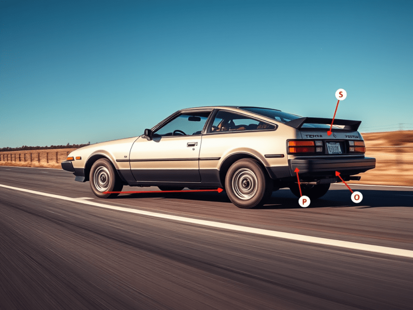
The Figure at the cover of this article is a Toyota Celica, model year 1981. There are three points highlighted in the cover Figure, S, P and O. These represents where there are pressure probes, these are estrategically displaced to evaluate pressure, speed and boundary layer when the vehicle is traveling at constant speed. This article will demonstrates how to calculate the speed, the lift and the drag components due to the aerodynamics.

Assumptions

• The Celica is traveling at constant speed and in a straight line path;
• The pressure probes devilever the following pressures p_∞ = 101000 Pa, p_s = 101240 Pa and p_p = 100700 Pa;
• The fastback stile of this Celica has a rear window with a slope φ = 18^∘;
• The trunk lid region has a length of 1.33 m and a width of 0.9 m;
• The C_f due to the air viscosity at the trunk lid region is C_f = 7.0×10^-5.

Objectives

1. To calculate the vehicle velocity;
2. To estimate the air velocity at the point p at a vertical distance normal to the vehicle roof;
3. To calculate the pressure coefficient at the point P;
4. To calculate the lift component due to the pressure distribution at the trunk lid;
5. To calculate the drag component due to the pressure distribution at the trunk lid;
6. To calculate the moment due to the pressure distribution at the trunk lid;
7. To calculate the lift component due to the viscosity effects at the trunk lid with C_f given.

Calculating the vehicle speed

The data previously presented allows to calculate the speed, but it is necessary an understanding of how is the air flow behaves over the vehicle. Figure 1 it is a good example to understand this.

As can be seen, there two Audi 100 from different model years and eight pressure probes positioned over the vehicle body. They are strategically positioned to evaluate the effect of the aesthetical changes in the vehicle design. For the Celica’s analisis in this article, the points S, P and O are similar to the points 5, 20 and 30 from Figure 1. The graph in this one indicates that at 5 there is C_p = 1, this occurs because this is an estagnation point where the air speed is basically zero. In any vehicle, this is the zone of highest pressure. Along the there is a great increase in the speed, but the region of the windshield this speed is decreases. It is possible to observe that C_p subtle decreases and start to increase in the region of the probe 15. The Audi 100 III exhibits a lower pressure decay at this region. This avoids separation, because a lower slope consume less mechanical energy of the flow at that point. The probe 20 register the lowest C_p obtained in both models. In fact, that zone of the roof in a road car is the one that the air speed is at maximum. It is also characterized by a great separation of the air flow. The optimized slope of the windshield helps to improve the mechanical energy of the air flow, which reduces the separation. Finally, at probe 30 it is possible to visualize that the difference between two vehicle is minimum. Actually, at this zone and beyond it is difficult to interpret the results due to the viscosity in this region. Therefore, it is possible recognize one condition for the Celica’s analysis. First, at the probe S, the speed (u_s) will be zero. Applying the Bernoulli theorem:

(p_∞/ρ) + (u_∞²/2) = (p_s/ρ) +(u_s²/2)

Since u_s = 0 and ρ = 1.2 kg/m³:

(p_∞/ρ) + (u_∞²/2) = (p_s/ρ)

u_∞ = √{2×[(p_s/ρ) – (p_∞/ρ)]}

u_∞ = √{2×[(101240/1.2) – (101000/1.2)]}

u_∞ = 20 m/s

Velocity at point P

Using the same procedure of the previous topic, it is possible to calculate the air velocity at point P. Again, this point is important, because it usually is the highest speed point. Hence, applying Bernoulli theorem:

(p_p/ρ) + (u_p²/2) = (p_s/ρ) + (u_s²/2)

(p_p/ρ) + (u_p²/2) = (p_s/ρ)

(u_p²/2) = (p_s/ρ) – (p_p/ρ)

u_p = √{2×[(p_s/ρ) – (p_p/ρ)]}

u_p = √{2×[(101240/1.2) – (100700/1.2)}

u_p = 30 m/s

Pressure coefficient at point P

Also using the Bernoulli theorem it is possible to calculate the pressure coefficient at point P. In fact, C_p is the main coefficient in the evaluation of a road and race car aerodynamics.

C_p = (p_p – p_∞)/q_∞ ; q_∞ = (1/2)∙u_∞²∙ρ

C_p = (100700 – 101000)/[(1/2)∙20²∙1.2]

C_p = – 1.25

As can be seen, Cp at point is very low which suggest a great loss of downforce and a great separation of the boundary layer at that region. Actually, the windshield slope and the transition of the end of the hood and the beginning windshield are very important to define with how much energy the flow will reach the roof of the car. This is the highest speed point even though the design of the windshield is optimized to reduce the separation at this region.

The effect of the rear window slope

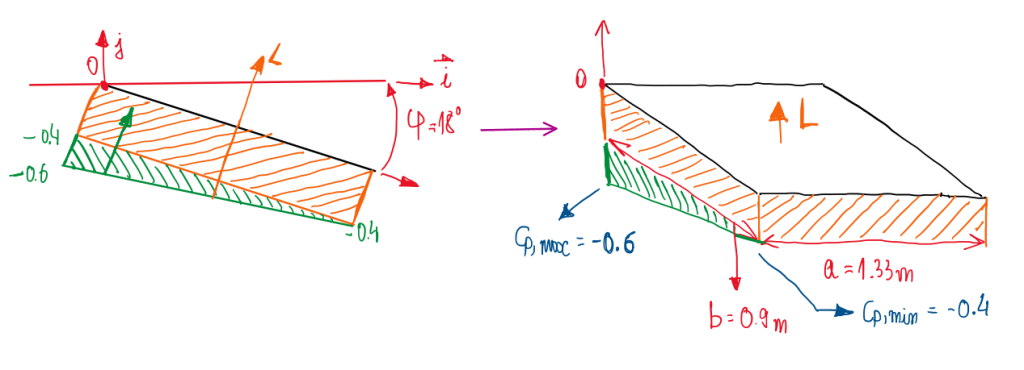
Figure 2 illustrates the inclination of the trunk lid and the reference system. In addition, it is possible to visualize the lift component due to the pressure distribution at the region. At this one Cp variates from -0.6 to -0.4, in other words, at the back of the Celica there is significant lifting compoent. Hence, it is possible to calculate it using the theories about the drag of slender and blunt bodies. The equation of the relative pressure:

F_p = – ∫_s C_p∙q_∞∙n dS → L = – ∫C_p∙q_∞∙j∙n dS = -C_p∙q_∞∙∫j∙ndS = – C_p∙q_∞∙∫cosφdS = -C_p∙q_∞∙cosφ∫dS

L = -C_p∙q_∞∙cosφ∙a∙b

C_p = (C_p,max – C_p,min)/2 = (-0.6 + (-0.4))/2 = -0.5

q_∞ = (1/2)∙u∞²∙ρ = (1/2)∙20²∙1.2 = 240

L = – (-0.5)∙240∙cos18^∘∙1.33∙0.90 = 136.610 N

Using the same approach, it is possible to calculate the drag component due to the pressure distribution:

Fp = – ∫_s C_p∙q_∞∙ndS → D = ∫_s C_p∙q_∞∙i∙ndS = -C_p∙q_∞∙senφ∙a∙b

D = – (-0.5)∙240∙sen18^∘∙1.33∙0.90

D = 44.387 N

The lifting component also generates a moment around the point O as is illustrated at Figure 3:

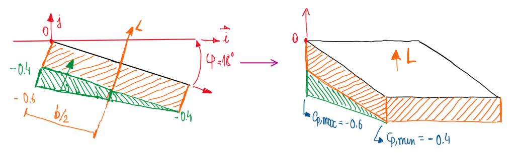
For this calculation it is possible to multiply the lifting component by the distance to the point O. However, there is another approach the account the pressure distribution due to C_p = -0.4 and the additional one that gives the maximum pressure coefficient, C_p = -0.6. This approach is similar the one seen in beam theory calculation for uniformly distributed loads. Hence, the equation for the moment around point O is written:

M_O = F_p∙(b/3) + F_p∙(b/2) = (-∫_s C_p∙q_∞j∙n dS∙(b/3)) + (-∫_s C_p∙q_∞j∙n dS∙(b/2))

M_O = -(C_p/2)∙q_∞j∙n∙(b/3)∙a∙b – C_p∙q_∞∙j∙n∙(b/2)

It is important to observe that there two C_p accounted in this calculation, C_p = – 0.4 and Cp = – 0.2, because there is a parcel of C_p add to the uniform C_p = -0.4. In this part, the resultant lifting component will be at the middle of the trunk lid, while the C_p = -0.2 will be at one third of b. In addition, this Cp is divided by 2, thus:

M_O = – (-0.2/2)∙240∙cos18^∘∙(0.90/3)∙1.33∙0.90 – (-0.4)∙240∙cos18^∘∙(0.90/2)∙1.33∙0.90

M_O = 8.197 + 49.18

M_O = 57.377 Nm

Together with the effects due to pressure distribution there is also the one due to the friction between the air and the surface, thus it is possible to calculate the lifting component due to the air viscosity.

Figure 4 illustrates that L_vis is the lifiting component due to the air viscosity is a negative one, thus it is a downforce. Hence, it is possible to calculate:

c_f(x) = τ_x(x)/q_∞

L_vis = τ_x(x)∙sinφ = q_∞∙C_f∙sinφ∙a∙b

L_vis = 240∙7×10^-5∙sin18^∘∙1.33∙0.90

L_vis = – 6.214×10^-3 N

As can be seen, the viscous component are not significant in terms of lifting.

References

1. W.H. Hucho, editor. Aerodynamics of Road Vehicles. SAE International, Warrendale, USA, 4th edition, 2002;
2. Stalio, Enrico. Aerodynamics. October, 2021.