The tire reference system illustrates how a wheel has several velocities. A three dimensional model is characterized by three axis, x, y and z. The first one is positive when pointing forward, while y and z axis are positive if pointing to outside and down from the wheel center, respectively. However, a car wheel is not positioned straight vertical, actually there is a small angle between the center of the wheel and the z axis, this is called, camber angle. The wheel can perform moments around two axis, the y and z axis, which are the rolling resistance moment M_y and the self-aligning torque M_z, respectively (Figure 1). There is also the over-turning moment, which around the x axis, but it is not commonly referred in the literature.

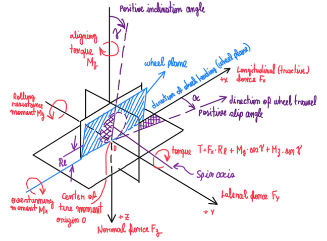
Although the rolling resistance moment affects the wheel rotation, actually the wheel rotates around its own axis which is able to move according to the wheel vertical travel. Since this also results in a camber variation, the torque demand over the wheel is always changing. The wheel spin axis moves according to the forces in x, y and z directions, thus it always changes its orientation. Hence, it is possible to calculate the torque demand:

T = F_x∙R_l + M_y∙cosγ + Mz∙sinγ

There is another important angle on tires operation, the slip angle α. This is the difference between the wheel travel and the direction of the wheel center line (wheel plane). α has a huge importance since the tire forces and moments are consequence of slip speed, which is the velocity component that is generated due to α. Another effect of the slip angle is the tire deflections, which is sometimes wrongly considered as the cause of tire forces and moments.

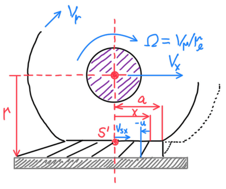
However, the tire deflection has some effects on tire operation. Actually, due to the contact patch deflection, there are some radii accounted in the tire calculations. The wheel radius is also called free unloaded radius r_f, because it is basically the wheel radius without any load over the tire. The rolling radius or loaded radius r is highlighted by the C point at Figure 2. It is basically the resultant radius after the tire deformation. Another important tire radius is the effective rolling one (r_e), which is described by the point S at Figure 2. This is characterized by its constant variation, thus a helical path is created as the car travels. In addition, the value of this radius is usually higher than the loaded radius, in other words, r_e is below the contact patch.

The main difference between the modern wheels and the old ones is the compliance. Nowadays automotive wheels deflect and provide a different contact patch geometry relative to the old rigid wheel, which has a contact patch basically defined by a line. Therefore, the free rolling conditions are also different, because the tire deflection result in a non-uniform contact patch and the resultant normal force F_z will be slightly displaced from the wheel (rim) center. This creates a torque component that acts against the wheel rotation, which is called rolling resistance M_y. In addition, the longitudinal force F_x will also be affected by this deflection, since it is a function of the off-set e_x (Figure 4).

As can be seen, F_z will generate a counter-rotation torque. e_x is due to the tire contact patch uniformity. Hence, it is possible to define some assumptions due to tire compliance. Since, the wheel rim speed is given by:

V_x = V∙cos(α) → Ω_x = 0

V_y = -V∙sin(α)

Ω_y = Ω

V_z = 0

Ω_z = 0

The effect of the slip angle must be better understood to provide a deeply definition of these velocities.

Slip angle and slip coefficient definitions

Basically, the slip angle is the difference between the direction which the wheel is pointing and the direction which the wheel is traveling and usually given by α. However, there are also the slip angles given by the velocity vectors which characterize the practical and the theoretical slip angle coefficient (Figure 5). Hence these two can be written by the following relations:

k_y = V_sy / V_sx

s_y = V_sy / V_r

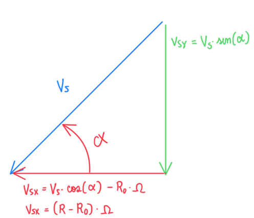
However, if the slip speed vector is deeply investigated (Figure 6) it is possible to visualize that the x component of the slip speed V_sx is a function of loaded and rolling radius. In other words, the tire deflection defines the slip speed vector, but this deflection is defined by the wheel loads. Since the vehicle is constantly exposed to load transfers, the slip angle is also at constant variation. Hence, it is possible to write the equations for V_sx and V_sy:

V_sx = (r – r₀)∙Ω = V_s∙cos(alpha) – r₀∙Ω

V_sy = – Vs∙sin(α) = – V_sx∙tan(α)

Hence, it is possible to update the equations of the theoretical and practical slip angles:

k_y = V_sy/V_sx = (V_sx∙tan(α))/V_sx = tan(α) → k_y = tan(α)

s_y = V_sy/V_r = V_sx∙tan(α)/V_r = (V_sy/V_r)∙tan(α) → s_y = (V_sy/V_r)∙k_y

Applying this concept for the longitudinal movements it is possible verify the slip coefficient:

k_x = – (V_x – Ω*r_e)/V_x

s_x = – V_sx / V_r = – (V_x – V_r) / V_r

References

• Guiggiani, Massimo. The Science of Vehicle Dynamics. Handling, Braking, and Ride of Road and Race Cars. New York, Springer, 2014;
• Reza N Jazar , “Vehicle Dynamics. Theory and Application”, Springer, 2008.