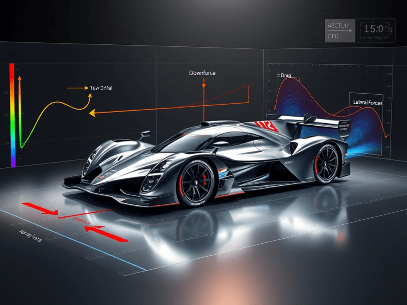
The setup of the model is done according to what the analyst wants to evaluate. The main parameter monitored are the aerodynamic forces, the pressure and the cooling. Usually, aerodynamic forces are monitored respective to a reference system, which it is possible to decompose the downforce, the drag and the lateral forces.

Aerodynamics loads

The aerodynamic loads are based on the integral along all the pressure boundaries of the car. These are decomposed according to the reference frame of the simulation. Actually, when simulating a car there are two reference frames, the one that refers to the position of the car and the other that is the wind axis.

for each boundary face i, P_i → F_i = ∫_A P_i∙n_i∙dA = P_i∙A_i∙n_i

This last one is particularly important, because during simulation the car is always hold aligned with x-global reference frame, which the floor is always aligned to the reference frame, then the simulation domain is inclined in order to impose the rake of the car. Hence, according to the ride heights of the car the domain it has a specific inclination. The wind inclination is definitive for the calculation of the aerodynamic forces and their decomposition in downforce and drag by the integral. This slope is defined respective to the global reference frame (Figure 1).

The aerodynamic forces are usually used in normalized values of these forces, because these are better to compare and to evaluate different situations. The normalized parameters are calculated by dividing the force or the moment by the dynamic pressure and the reference area. In the case of moments, the reference area and length are multiplied together with the dynamic pressure.

C_d = F_x / (q_∞∙S_ref) ; C_l = F_z / (q_∞∙S_ref) ; C_m = M_y / (q_∞∙S_ref∙L_ref) ; q = ρ_ref∙V²/2

The reference parameters are important points of these calculations. Usually, the reference area S_ref is assumed equal to 0.5, because most of racing car CFD simulations are performed with the CFD model splitted in two symmetrical parts (Figure 2). Some runs are performed with the entire model, thus S_ref is assumed as equal to 1. The reference length, L_ref, is assumed as the vehicle wheelbase.

The most important reference parameter is the free stream velocity, usually given by U_∞ = 50 m/s. This values is adopted considering that the flow is incompressible. It is a safer approach, because it guarantees a good accuracy when comparing and evaluating the coefficients. However, since in reality the Reynolds number does not change in a quadratic way, this approach is not 100% safer.

Cooling

In terms of cooling, the solver process deals with the target that the cooling system should reach. These are the velocity crossing the radiator surface. It is not possible to monitor the ratio between the cross velocity through the radiator and the reference velocity, which is expressed through a percentage. For instance, a radiator has 30% crossing velocity, thus the velocity at the inflow is 0.30∙V_ref. Another parameter which is easy computed by CFD softwares is the mass flow rate entering the body divided by the free stream mass flow.

V_r/V_ref = m’/(ρ_ref∙A_r∙V_ref)

Many correlation data are obtained from the wind tunnel and track testing, since it is used in many sensors and automated structures. In CFD it is also possible to check the airflow at the parts and sections of the bodywork. The big advantage of the CFD environment is that there is more continuity of the pressure, velocity or any other parameter crossing the domain.

This is not the case for other kinds of experiments. For instance, simulations like the pressure tap acquisition from the wind tunnel, it is possible to set on the CFD software the coordinates of the pressure taps added on the other experiments. Hence, it is possible to import data of the same project, but from different environments and use them to feed the CFD solver with validated data. This is an optional approach since it requires a complete chain of experiment environments.

Simulation

When the convergence of the simulation is reached, the monitor shows a situation similar to the one at Figure 5. This occurs, because the solver is iterative. Each iteration has a different value, if it is plotted against the number of iteration, the monitor will exhibit that there are some fluctuations about the average value. Considering the downforce, the output of this parameter is really dependent of the number of iterations in which the simulation is stopped. If the simulation is pretty well converged, thus the iteration value will not significative change. However, this not always occurs, in some situations the convergence takes more time. In these cases, the monitor is useful to evaluate when stop the convergence. The safest choice is to average a certain number of iteration. The averaging not only account the output values, but also all variables in all the cells, then it is allowed to output the averaged variables of these cells. Hence, the solver equations enter in a loop, which is the iterative solver until reach the convergence. It starts from the previous solution, then iteration by iteration it reads the boundary condition, the solver discretizes the incompressible NSE in a finite volume discretization and check if the iteration is converged. When the iteration did not converge, another iteration is ran. There are metrics that indicate if the iteration is converged or not, that are the residuals.

Residuals

These are metrics that exhibits quantitatively how good is the iteration that was converged. There is one residual for each solved equation. Since incompressible NSE and laminar are the base of race car simulations, thus there are 4 residuals, 1 for the continuity equations and 3 for the momentum equations. The lower the residuals, the better the iteration solution, thus the convergence. The residuals are characterized as good when it starts from a particular value, decrease and then reach very small differences, almost a constant value. The reduction for a good residual is at a magnitude order 10^-3. This occurs, because at some point, the iterative solver is not able to solve better the equations, for this reason the residuals became constant or have very small differences.

Analyzing residuals

A typical plot for a good residual is illustrated at Figure 6. There are 6 residuals, which 3 of them are for the velocities and 1 for the continuum equation. In addition there are other 2 for the turbulence model k-ξ. Hence, there are residuals for the kinetic energy and turbulence intensity. As can be seen, most of the residuals start from a value, then after four hundred iterations, the process reaches a pretty constant number of residuals values, that are at an order of magnitude of 10^-3.

Figure 7 illustrates that 400-500 iterations are sufficient to obtain well converged iterations. The main objective of the solver, respective to the residuals, is that these should be reduced to an order 10^-3 in few iterations and at some point stabilizes its value. A similar consideration can be applied to the quantities which are being monitored. For instance, if the solution is converged, it is expected that the performance parameters which are being monitored reach stable values, without fluctuations around the average. A good strategy is to avoid this is to plot all the monitored parameters across the iteration number, as in Figure 5, and qualitatively access the reached average value during the last solver. Another option is to use more deterministic criteria. For instance, to compute the slope of the plot across the iteration number that will be averaged and the standard deviation. For example, Figure 8 illustrates these parameters, it gives a more objective criteria to choose when the monitored parameters are converged.

Once with these metrics, organize them in plots and tables helps to evaluate the solver process. These contains the averaged value and the slope. As can be seen, the slope is very low and it can be considered that the simulation converged by this value (0.0006). In addition, the same type of evaluation, by the slope, can be applied to all other parameters and also for different ratios. For instance, different parts of the car can obtain or not the convergence. The car is split in different parts and these are plotted in those different metrics for these sections of the car. Hence, it is possible to understand which of them is slower to converge.

Reference

• This is article is based on the lecture notes taken by the author during the Industrial Aerodynamics lectures hold by Muner at Dallara Accademy.