When evaluating the vehicle aerodynamics, an important theory behind the effect of wing and the flat underbody is the boundary layer theory. As can be seen in the Figure at the cover of this article, the flat plate is immersed in an airflow that a has a free stream velocity U∞, the origin of the coordinate system coincide with the leading edge of the flat plate. The boundary layer is the term given to the airflow area which the profile is non-uniform in the vertical and normal to the wall direction. Two kids of regime are observed, laminar and turbulent one. Laminar flows are functions of the coordinates, thus u = u(x,y), while turbulent flows are functions of the three coordinates and also the time, thus u = u(x,y,z,t) or <u>(x,y). This last one is adopted when it is not possible to analyze a so irregular profile. For this, the time base is adopted. The boundary layer is a region of the space which has a thickness given by δ(x) and the velocity inside the boundary layer in 99% of the free stream velocity U_∞. Hence, the following characteristics can be summarized:

Dimensional analysis

The boundary layer theory is based in Prandtl considerations, which through the analysis of the magnitude order it was defined that the energy balance advective and viscous term have the same order of magnitude.

u(∂u/∂x) ~ ν(U_∞/δ²)

From the derivative definition, it is possible to write the advective terms:

and the viscous terms

∂²u/∂y² ~ U_∞/δ²

Hence, this correlation become:

u(∂u/∂x) ~ ν(U_∞/δ²) → δ² ~ x²/Re_x → δ ~ x/√Re_x

Later, Blasius proposes that for a laminar flow, the boundary layer thickness would be given by:

δ(x) = 4.91∙(x/√Re_x) ≃ 5x/√Re_x ; Rex ≡ U_∞∙x/ν

This means that the boundary layer thickness is proportional to the square radius of the reference length, which its values depends of the application.

For a better understanding, it is possible to apply this theory to a simple automotive case, which a road car is traveling at 15 m/s. A boundary layer develops along the vehicle roof and reach some value at 1 m. Considering ν = 15∙10-6 m²/s, the boundary layer thickness is:

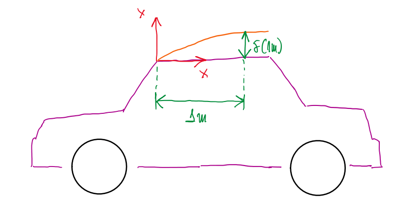
Rex ≡ U_∞∙x/ν = 15∙1/15∙10^-6 = 1000000 → Laminar

δ = 4.91∙/√10⁶ = 4.91∙10^-3 = 4.91 mm

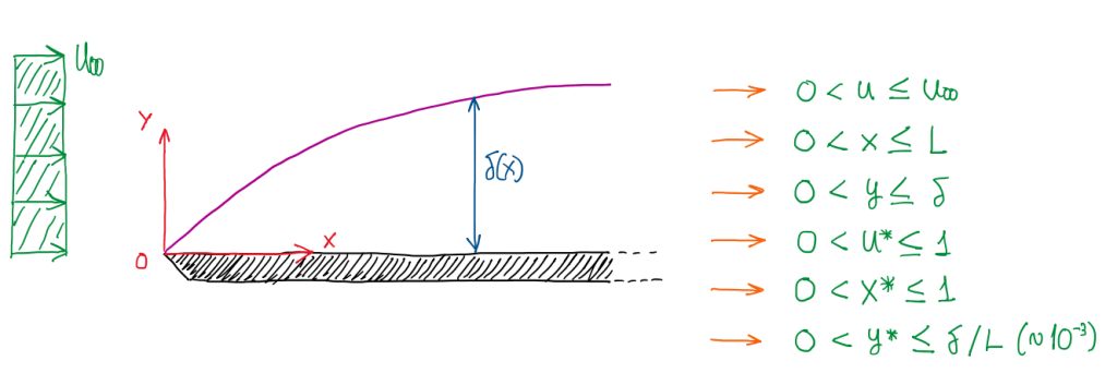
This simple exercise suggests that for 1 m length, a boundary layer thickness developed is just 4.91 mm. In other words, the boundary is long and thin. Another important conclusion about the dimensional analysis is that boundary layer thickness has the same order of magnitude that the characteristic length divided by 1000 (δ ~ L∙10^-3). However, this last conclusion refers to the automotive applications. A laminar flow is characterized by its two dimensions, because it is stationary (∂*/∂t = 0), this make those calculations more easy to be described. Even though, this can also be applied for turbulent cases. Since the transient nature of this one, it is interesting to introduce reference dimensions:

m → L : Boundary layer length

kg → ρ_ref : Reference density (ρ = constant)

s → U_ref = U_∞ : Free stream velocity

The first step is to normalize the mass conservation equations (ρ = constant):

∂u/∂x + ∂u/∂y = 0 → (L/U_∞)∙(∂u/∂x + ∂u/∂y) = 0 → ∂u*/∂x* + ∂u*/∂y* ; u* ≡ u/U_∞ , x* ≡ x/L

Thus, the partial derivative can be given by:

du/dx = lim_{Δx → 0} [u(x + Δx) – u(x)]/Δx → (du/dx) ~ (U_∞/L)

Inside the boundary layer:

After normalized the main parameters, it is possible to write:

u* ~ 1 ; x* ~1 → ∂u*/∂x* ~ 1 ; y* ~ 10^-3

y ~ 10^-3 → v* ~ 10^-3 → ∂v*/∂y* ~ 1

∂u*/∂x* + ∂v*/∂y* = 0

Hence, the order of magnitude of these variables can be measured:

Δu* ~ 1 ; Δx* ~ 1 ; Δv* ~ ∂/L ; Δy* ~ ∂/L

References

• Stalio, Enrico. Aerodynamics. October, 2021;

• http://www.aerodinamica.unimore.it