When analyzing the vehicle aerodynamics there are some situations that the it is difficult to properly describe the flow. A solution for this is called potential flows, theoretical elementary flows that can be combined between themselves to replicate a complex real flow. Although potential flows have some limitations, they are good approximations to real flows.

Characteristics

The main hypothesis of potential flows is that the flow is constant density and irrotational. Another characteristics are summarized below:

grad[(∂φ/∂t) + (P/ρ) + (v²/2) + g∙h] = 0

The velocity field v is already known through the Laplace equations, the derived form relative to time accounts the past condition. The main differences between the potential flows and Navier-Stokes Equations (NSE) are summarized in Figure 1.

The coupling characteristics refer to the equation coupling. For instance, NSE can be coupled with other equations, while potential flow equations can be solved decoupled form the Bernoulli equation. In terms of superposition, the solutions can be superposed or not. NSE does not allow superposition, while potential flow does, except for pressure. The reason is described below:

∂φ/∂t + P/ρ + (gradφ)²/2 + g∙h = ζ(t)

grad φ = v

v₁² + v₂² ≠ (v₁ + v₂)²

Finally, the external-internal condition refers to the difference between these flows.

Potential and stream functions

The potential flow field v can be defined by cartesian and cylindrical coordinates. The cartesian coordinates are summarized below:

grad φ = v

v = (u,v) = (∂φ/∂x , ∂φ/∂y) → Cartesian coordinate potential flow field

v = (u,v) = (∂ψ/∂y , – ∂ψ/∂x) → Cartesian coordinate stream function

The cylindrical coordinates are summarized below:

grad φ = v

v = (u_r,u_θ) = (∂φ/∂r , (1/r)∙(∂φ/∂θ)) → Cylindrical coordinate potential flow field

v = (u_r,u_θ) = ((1/r)∙(∂ψ/∂θ) , – ∂ψ/∂r) → Cylindrical coordinate stream function

Figure 2 illustrates a graphical representation of these equations.

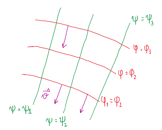
As can be seen, the velocity field is perpendicular to the lines of the potential flow field. This allows to write:

v = ((1/r)∙(∂ψ/∂θ) , -∂ψ/∂r)

grad ψ = (∂ψ/∂r , -(1/r)∙(∂ψ/∂θ))

These are the equation that describes the grad ψ ⟂ grad φ. The iso-lines of the stream function are perpendicular to the potential lines function and the stream function isolines are always parallel to the velocity field, thus it is possible to write:

gradφ ∙ gradψ = (u,v)∙(-v,u) = 0

Potential flow solutions

Since the Laplace equations are linear, the superposition of effects can be structured in order to simplify the calculation. These are the elementary flows which can be summed between them.

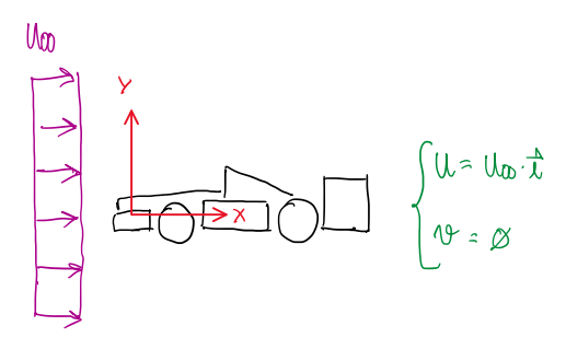
Uniform flow

div(v) = 0

curl(v) = 0

v = (∂φ/∂x , – ∂φ/∂y) = (U_∞ , 0)

φ = φ(x,y) = ∂φ/∂x = U∞ ; ∂φ/∂y = 0

Beginning with the potential function:

∂φ/∂x = U_∞ → dφ/dx = U_∞ → ∫dφ= ∫U_∞dx

φ = U_∞∙x + c = U_∞∙x

Since the potential function only has a physical meaning when in form of gradient and c is an arbitrary constant, it can be assumed that c = 0. For the stream function the same procedure can be applied:

v = (∂ψ/∂y , – ∂ψ/∂x) = (U_∞ , 0)

ψ = ψ(x,y) = ∂ψ/∂y = U_∞ ; ∂ψ/∂x = 0

∂ψ/∂y = U_∞ → dψ/dy = U_∞ → ∫dψ= ∫U_∞dy

ψ = U_∞∙y + c = U_∞∙y

Hence, it is possible to conclude that uniform flows are given by two equations:

φ = U_∞∙x
ψ = U_∞∙y

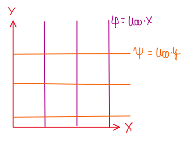
The uniform flow is graphically represented as illustrated by Figure 4. As can be seen, the calculations described that the potential functions are perpendicular the stream functions.

Elementary vortex

v = (u_r,u_θ) = (0 , Γ/(2πr))

div(v) = (1/r)[∂(u_r∙r)/∂r + ∂u_θ/∂θ] = 0

curl(v) = 0

v = (∂ψ/r∂θ , – ∂ψ/∂r) = (0, Γ/(2πr))

Thus:

∂ψ/r∂θ = 0

-∂ψ/∂r = Γ/(2πr) → dψ/dr = -Γ/(2πr) → ∫dψ = -(Γ/2πr)∫dr → ψ = -(Γ/2π)∙ln(r) + c

ψ = -(Γ/2π)∙ln(r)

Usually adopted:

ψ = -(Γ/2π)∙ln(r/R)

The potential function can be integrated by the same procedure:

v = (∂φ/∂r , ∂φ/r∂θ) = (0 , Γ/2πr)

∂φ/∂r = 0 ; ∂φ/r∂θ = (Γ/2πr)

∂φ/r∂θ = (Γ/2πr) → dφ/dθ = (Γ/2π) → ∫dφ = (Γ/2π)∫dθ → φ = θΓ/2π + c

Finally, it is possible to write both equations for the elementary vortex and its graphical representation, which is illustrated at Figure #.

φ = θΓ/2π + c
ψ = -(Γ/2π)∙ln(r/R)

As can be seen, the elementary vortex has two components, the stream function, that results in the circular structure with a constant radius, and the potential field component, which is given by a circular disposed lines at constant angles.

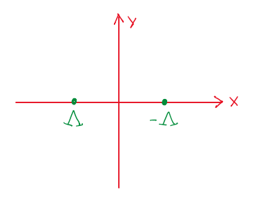
Source

v = (u_r,u_θ) = (Λ/2πr , 0)

v = (∂ψ/r∂θ,-∂ψ/∂r) = (Λ/2πr , 0)

thus, integrating the terms:

∂ψ/r∂θ = Λ/2πr → ∂ψ = Λ/2π∫dθ → ψ = Λθ/2π + c → ψ = Λθ/2π

∂ψ/∂r = 0

thus, the velocity field of the source is given by:

ψ = Λθ/2π
∂ψ/∂r = 0

As can be seen, the source has several stream functions lines that arise from the origin at the center of the cylinder. They are not tangent to the circle since the tangential velocity u_θ is null.

Elementary flows combination

The importance of the potential flow is that hey can be used to study some types of flows which are difficult to reproduce. For this reason, there are many elementary flows, which are combined to reproduce some kind of flow which is not common. An example is combining the uniform and the source elementary flows as described below:

ψ_uniform = U_∞∙y = U_∞∙r∙sinθ

ψ_source = Λθ/2π

Thus the stream function is:

ψ = Λθ/2π + U_∞∙r∙sinθ

The velocity field is given by:

v – (u_r,u_θ) = (∂ψ/r∂θ, – ∂ψ/∂r)

u_r = ∂ψ/r∂θ → u_r = r^-1[Λ/2π + U_∞∙r∙cosθ]

u_θ = – ∂ψ/∂r → u_θ = U_∞∙sinθ

The velocity field of the non-lifting flow around a cylinder is:

u_r = r^-1[Λ/2π + U_∞∙r∙cosθ]
u_θ = U_∞∙sinθ

The main characteristic of this flow is the stagnation points, which is described by v = 0:

v = (u_r,u_θ) = 0

u_r = r^-1[Λ/2π + U_∞∙r∙cosθ] = 0 → Λ/2π + U_∞∙r∙cosθ = 0

u_θ = U_∞∙sinθ = 0 → U_∞∙sinθ = 0 → sinθ = 0 → θ = ∅ + k∙π ; k = 0,1,2,…

Now it is possible to update u_r

(Λ/2π + U_∞∙r∙cosθ)|_{∅ + k∙π} = Λ/2π – U_∞∙r = 0 ; θ = π

Λ/2π = U_∞∙r → r = Λ/(2π∙U_∞)

Assuming that r > 0, the only solution for u_r = 0 is with cosθ being a negative value, thus the value of k must be an odd integer number. Graphically, the result is represented by Figure 6:

As can be seen, if r_s increases, U_∞ decreases, conversely if r_s decreases, U_∞ increases. This means, that the separation points become near to the origin. The interesting point is that the separation line can be considered a solid body. Hence, this could be a wing or an aerodynamics device. This is possible, because by definition, the stream lines of the velocity are always parallel to the separation stream lines. In addition, it is possible to consider the separation stream line as a solid body, but with the source being an internal flow.

Rankine oval and doublet

Another important potential flow combinations are the ranking oval and the doublet. The Rankine oval is a sum of the uniform flow with the source and the sin, which results in the following structure:

An interesting point about the Rankine oval is that if the source and sink get very near each other, it is possible to create a 2D cylinder. Hence, it can be useful to create potential flows that emulates cylinder aerodynamics. The doublet potential flow is defined by a source and sink of equal strength Λ, thus:

The strength of the doublet is defined as:

lim_d→0 Λ∙d = k [m³/s]

The stream function is given by:

ψ = – k∙sinθ/2π∙r

Hence, the doublet is illustrated by Figure 9:

The constant lines are circumferences of a diameter defined as k/2πψ.

Non-lifting flow over circular cylinder

Since the main elementary flows are already described and that is is possible to combine them to emulate different flows, one of the main cases is the non-lifting flow over a cylinder. In this case two potential flows are used, the doublet and the uniform flows.

ψ_doublet = – k∙sinθ/2π∙r

ψ_uniform = U_∞∙r∙sinθ

ψ = ψ_doublet + ψ_uniform = – k∙sinθ/2π∙r + U_∞∙r∙sinθ = U_∞∙r∙sinθ[1 – k∙/2π∙U_∞∙r²]

Considering R² = k∙/2πU_∞:

ψ = U_∞∙r∙sinθ[1 – R²/r²]

ψ = U_∞∙r∙sinθ – U_∞∙R²∙sinθ/r

Hence, applying the definition of the potential flow:

v = (ur,uθ) = (∂ψ/r∂θ,-∂ψ∂r)

u_r = ∂ψ/r∂θ = U_∞∙cosθ[1 – R²/r²] ; R = √k/2πU_∞

u_θ = -∂ψ∂r = -U_∞∙r∙sinθ(1 + R²/r²)

Hence, the velocity field of non-lifting flow around a cylinder is:

u_r = U_∞∙cosθ[1 – R²/r²]
u_θ = -U_∞∙sinθ(1 + R²/r²)

Analyzing both tangent and radial velocities it is possible to write some conclusions about them:

u_r = U_∞∙cosθ[1 – R²/r²] ; u_r → 0 when r → R

As can be seen, the radial velocity goes to zero if the circumference radius r equals to R. Hence, the flow will only exhibit the tangential velocity and the circumference is a separation stream line, thus there are stagnations points. These are given by ψ = (u_r,u_θ) = (0,0), thus:

ψ = (u_r,u_θ) = (0,0)

u_θ = -U_∞∙sinθ(1 + R²/r²) = 0 → sinθ = 0 ; θ = 0, π

Hence, the stagnation points are (R,∅) and (R,π) as illustrated by Figure 10:

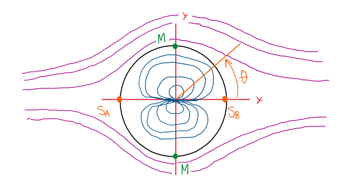
The flow lines are symmetric relative to the x and y axis and the lines of the cylinder can be considered as a solid body. However, it is important to notice that, even though u_r is zero due to r = R, the tangential velocity changes according to θ:

u_θ = -U_∞∙r∙sinθ(1 + R²/r²) → u_θ = -U_∞∙sinθ(1 + 1) → u_θ = -2U_∞∙sinθ

u_θ = -2U_∞∙sinθ

Hence, the velocity will be maximum when θ admit values ½π or 3π/2, which results:

u_θ|_max = 2U_∞

Therefore, it is possible to visualize that in potential flows, there is no tangential stress, thus viscosity is not an important parameter. However, there are normal stresses associated to the deviatoric tensor. Hence, the pressure distribution is a support to describe the force due to pressure. In addition, this case allows the use of the strong form of the Bernoulli equations to derive the pressure coefficient:

p + ½ρu² = constant → p + ½ρu² = p_∞ + ½ρU_∞²

p – p_∞ = ½ρU_∞² – p + ½ρu² ; u = ∅

(p – p_∞) / q_∞ = 1 ; q_∞ = ½ρU_∞²

As can be verified, the difference between pressures is divided by the dynamic pressure q_∞, which equals to 1. Actually, neither all cases are equal to 1, which require to calculate the pressure coefficient:

C_p = (p – p_∞)/q_∞

Where q_∞, the dynamic pressure and specific kinetic energy of the undisturbed flow. Hence, applying again the Bernoulli:

p + q = p_∞ + q_∞ → p – p_∞ = q_∞ – q → p – p_∞ = ½ρU_∞² – ½ρu² → p – p_∞ = ½ρU_∞²(1 – u²/U_∞²)

(p – p_∞)/½ρU_∞² = (1 – u²/U_∞²) → C_p = (1 – u²/U_∞²)

Now there are two equations for the pressure coefficient, but if it is being considered the strong form of the Bernoulli equation, thus it is correct to use:

C_p = (1 – u²/U_∞²)

Hence, applying those equations on the non-lifting flow over a cylinder, which the value of the pressure over the solid surface can be mapped. This is important, because is at the surface that forces act, thus from the previous calculations:

u_θ(r = R) = -2U_∞∙sinθ ; C_p = (1 – u²/U_∞²)

C_p = (1 – u²/U_∞²) = [1 – (2U_∞∙sinθ)²/U_∞²]

C_p = 1 – 4sin²(θ)

The pressure coefficient described above is the one applied at the surface of the cylinder as illustrated at Figure 11.

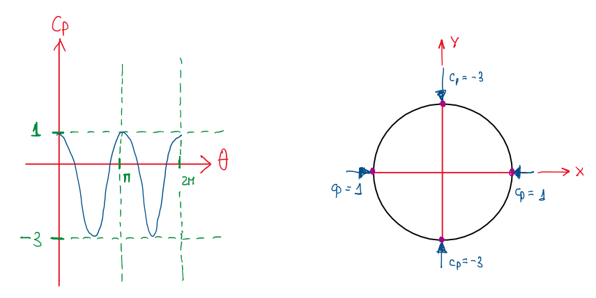
Hence, it is possible to visualize that the maximum C_p is 1 and it occurs at angles 0 and π. On the other had, the lowest C_p is -3, obtained at angle π/2 and 3π/2. The cylinder is exposed to axial efforts due to the pressure. The symmetry of the pressure coefficient over the surface balance the forces generated. If the cylinder is immersed in a flow, there is the possibility of lift or drag generation, thus a force is required to balance. However, the symmetry presented at the calculations demonstrated that it is self-balanced. This is called D’Alambert paradox. Actually, it must be understood that potential flows are accurate for streamlined bodies, but ias not suitable for blunt bodies. This is the reason why in race car wing studying, potential flows are considered.

Lifting flow over a circular cylinder

If an elementary vortex is summed to the previous flow, the new potential flow can be visualized through Figure 12.

In the last element, it was observed that there is a symmetry that result in a balanced force over the cylinder. However, adding a potential vortex to the non-lifting flow it is possible to visualize that the separation streamline is not displaced. This occurs, because the vortex streamlines are circumferences around the vortex center. Hence, the sum results in an identical line to the solid body line. The elementary vortex and the sum of this one with the non-lifting flow:

u_r = 0

u_θ = Γ/2πr

ψ = U_∞∙r∙sinθ(1 – R²/r²) – (Γ/2π)∙log(r/R)

The most important variable in those equations is the circulation Γ, it can exhibit infinite configurations. For instance, if Γ < 0, the stagnation point is displaced to the lower part of the cylinder. The stagnation stream lines are only symmetrical relative to the y-axis. Hence, due to this partial symmetry, the force component at ax direction due to pressure remains balanced. In addition, the velocity at the top of cylinder is lower than the one at the lower part of it. However, along the x-axis there is no symmetry, which results in a force that acts along the y direction. The main point of the case which Γ > 0, is that the velocity at the top of the cylinder is higher than the lower part. As a result, the non-lifting flow now become a lifting one. Actually, the circulation can assume different values, since there are infinite possibilities (Γ ∈ (-∞,∞)) for potential flows of a solid body. For each solution, there is an associated lift. Hence, when ∞ – 0, the lift is zero. These imposed conditions are a a little weak since they allow that an attached flow moves at a tangential direction. In other words, the only condition is the impermeability at the wall ∂φ/∂n|_w = 0. Frequently, it is defined that fixed cylinders have only one potential solution, while rotational cylinders admit infinite solutions. However, it is important to understand that potential flows do not distinguish between a fixed or a rotational cylinder. In real conditions, a rotational cylinder generates lift, thus the potential flow solution is a replication of the flow around a cylinder, but with influence of the velocity at the vicinity.

Potential flows around an expansion corner and in a sink

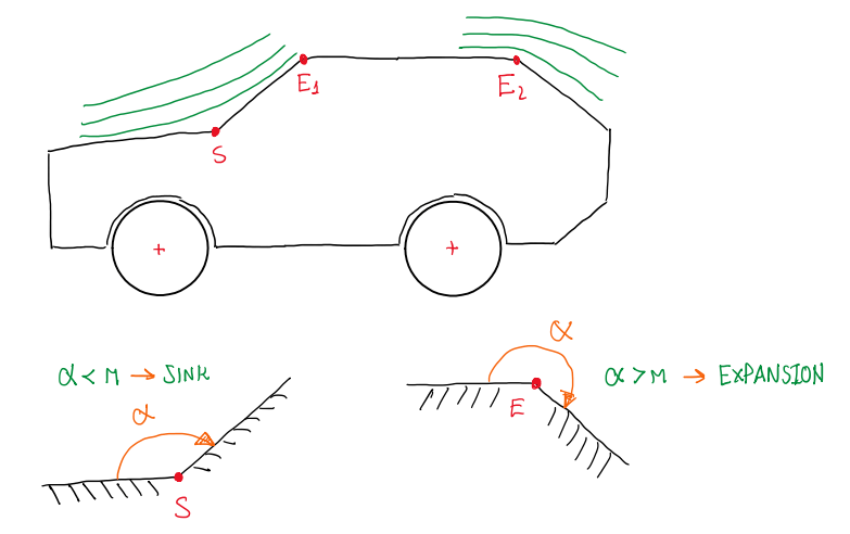
There are two important points along a vehicle body that can be analyzed by potential flows, one at the region between the end of the hood and the beginning of the windshield, the other is about the region of the tail gate or deck lid. Figure 13 illustrate the regions described as sink and expansion corners. Actually, these are concave and convex angular sections. The solenoidal irrotational flow exhibited at these two situations can be described by the Laplace equation under the condition that the normal velocity componet vanishes at the wall. Hence, the solution for these two cases are described by:

φ = A∙rⁿ∙cos(nθ) ; n = π/α

Understanding that this is given in polar coordinates and applying similar procedure as before, it is possible to write the velocity field v:

u_r = n∙A∙rⁿ∙cos(nθ)

u_θ = – n∙A∙rⁿ∙cos(nθ)

The polar coordinates has the reference center of the system at the points S and E. Hence, it is possible to analyze these cases. Considering the sink situation, from the point S to the point E, the distance is given by r and the angle is positive clockwise. Another parameter visualized at the velocity field equations is n, which is defined according to the situation.

n = π/α

n > 1 → (u_r,u_θ) → ∅ ; r → ∅ → Sink-Stagnation

n < 1 → (u_r,u_θ) → ∞ ; r → ∅ → Expansion Corner

An important point about these solutions is that the y differ of the real condition, because of the potential flow boundary conditions. In addition, the flow also behaves differently between sink and expansion. In the first, it is possible to observe that the stream lines tends to get away from the surface (Figure 13). For expansion corner sections, the opposite occurs, the stream lines tend to get near to the surface, thus the velocity tends to increase. The sink and the expansion cases usually occurs at regions between the hood and the windshield, the windshield and the roof, the roof and the tail gate. In race cars, this is commonly found in diffusers.

References

• Stalio, Enrico. Aerodynamics. October, 2021;
• http://www.aerodinamica.unimore.it