In any mechanical system, one of the main concerns is the failure or the collapse of the structure. The material engineering already stated the concepts of stress and deformations at the failure, thus the specific resistance of materials. However, the collapse of the structure does not necessarily coincides with the failure stress of the material. Hence, it is necessary to develop a rupture criteria after failure theory. This is a relation that accounts all loads and stresses for the material. In other words, is a process that defines what will be the strength and the stiffness before the material exist. This process is also called, virtual material design. Hence, the failure theory must be accurate, replicable and reliable. The objective is to have a solid information to be applied in simulations and testing. This information is also used for the sizing of the component that will be made from that material. Regarding the safety, the failure criteria allows to define the safety margin and the points of the component with the highest and the lowest strength. This is very useful for the material optimization for a specific shape, which allows the identification of the areas with low and high safety margin. Hence, in a further step, the development of a laminate to build a component with an even safety margin across its area is possible. This is the uniform resistance design. In practice, the component has shapes with an even safety margin across its area and an optimised strength to weight ratio. Unavoidably, all those aspects guide the development process of the material, because the failure criteria start on the micro-mechanics. Since the analysis of different multi-scales of the composite materials allow to correlate thickness and strength of the constituents, defining a failure theory for them allows to make materials for specific applications and components. All this process is called, virtual material design.

Failure criteria for composite materials

In terms of micro-mechanics, it was defined some properties for composite materials. Basically, these are heterogeneous, but they are assumed as isotropic, orthotropic and anisotropic. These are solutions to ease the calculations since composite materials are heterogenous and anisotropic ones. These mean that, the composite material properties vary according to the position across the laminate and loading directions, respectively. However, the failure criteria is a local analysis and, according to those characteristics, it can deliver different results. The solution for that is the behaviour homogeneization. This proposes that, the material homogeneity is incorporated into the material behaviour. Hence, the failure criteria is not in the micro-scale anymore. Instead of analyzing point-per-point or each constituent, the analysis if performed in a larger scale. There are no constituents into the material, just an homogenous one. Therefore, the properties do not vary along the laminate, but they do according to the loading conditions, thus the stress state. This is also called, anisotropism.

Anisotropic material

An anisotropic materials is characterized by strength independency with respect to the orientation of the stress state. In other words, each point of the material has the same strength. This is the reason why the calculated equivalent stress (tensile stress) is compared with the tensile strength, because in that case is enough. In the case of anisotropic material, the strength is a function of the stress field orientation with respect to the principal material direction. This is what it is possible to see qualitatively. For instance, a ply which is off-axis, then its strength is not the same because it was in the load direction. Therefore, for composite materials, what should be compared is not the stress in a direction with the maximum strength on that direction, rather the equivalent stress field should be compared with an allowable stress range for that stress field. This means that, this allowable stress range would not be an unique value as in the isotropic materials. Actually, it will be a value which is a function of the stress state at each material point. Hence, in anisotropic materials there is nor the shear stress neither the ultimate strain, but there is the equivalent stress and strength, which is dependent of the ply orientation.

Strength characterization

The strength characterization is based in five properties, which are characteristics of the material in the principal material direction. The properties are the tensile, the compressive and the shear strengths. The first two can occur in both directions (1 and 2). The shear strength occurs across the planes 1 and 2. Hence, due to those aspects, there are five parameters. These are accounted according to the ply orientation with respect to the loading condition. Then, the allowable stress state can be defined. The ply can be oriented with respect to the loading, thus longitudinally or transversally. In addition, it can also work in shear. Hence, there are three basic fiber-matrix working modes, longitudinally, transversally and shear strength. The main difference between these cases is that they can work in series or in parallel. This result in different effects on the laminate. Considering the longitudinal case, the ply and loading are aligned at the same direction. In this case, the tensile loading is well resisted, while the compressive one is not. This occurs due to the fiber local instability to compression. In the longitudinal case, the fibers and the matrix behave as they are in series. The transversal condition is characterized by the ply oriented at 90° with respect to loading. Usually, this condition is more related to the matrix, which works better when under compression loading than tensile one. The reason is that, in this configuration, they work in parallel link. If the matrix-fiber link is weak, normally the failure occurs at the matrix, because it is the weakest compound. When the transversal case is working in compression, the matrix and fibers work together creating a good resistance. This occurs, because of the relation between those compounds with respect to load transferring. However, it is necessary a balanced trade-off with respect to soft or hard matrices. An excessive soft matrix can let the fibers suffer some damage. This results in already damaged fibers before a great impact or energy absorption, thus reducing performance. The shear strength conditions occurs when the laminate is exposed to in-plane shear stresses. Even though the matrix and fibers work in series, the shear occurs at the matrix and has no influence of its sign. The reason is the symmetry of the shear stress field.

Failure criteria

Usually, there are two criteria to evaluate the failure theory, these are the micro-mechanical and the phenomenological ones. The first one is more complex regarding heterogenous materials. It can be adopted in cases which every material point is predicted at the lower limit of the matrix and fibers. The phenomenological criteria is very similar to the Von Mises one. In this case there is no prediction of the micro-mechanics of the material at failure, because the material is considered a homogeneized one at failure. The local micro-mechanics of the failure have no reason to be deeply known. The objective of this criteria is to obtain the stress limit curves or surfaces of the available stress in the material in order to compare that with the current stress state. Those limit curves and surfaces define the failure criteria, because they are the limit envelope of fracture. This definition is only valid for composite materials, because these have no plastic deformation. Instead of it, they basically break without significant plastic deformation. For this reason, most of composite materials are considered brittle. In the case of metals, the failure criteria would be the limit envelope of plasticity.

Hence, based on those aspects, many theories were developed in order to describe the failure criteria. They were split in two categories, the first-order and the interactive criteria. The first-order is also called non-interactive. The reason is that, it is based on the comparison of stress and/or strain state with the strength characterization properties. The first order criteria can be applied by two theories, the max stress or the max strain ones. The interactive criteria has many theories developed. The most commonly used are the Tsai-Hill, Tsai-Wu and Hoffman theories. The interactive criteria are polynomial functions of the stress state that uses the strength characterization properties as parameters.

In any case, the output of a failure criteria are two parameters. They describe if the laminate is prone to fail or not, these are the failure index (FI) and the strength ratio (SR). The failure index is a pass-fail fast checking parameter, it describes through a scalar value if the regions of the laminate are prone to fail or not. The threshold value is 1. If the failure index indicates values lower or equal to 1, then that region is working with some safety margin, thus is not prone to fail. Above that value, this material could fail. In general, the failure index should be adopted for cases which the theory is based in non-linear combinations of stresses. In addition, this approach can not be immediately used to deduce the allowable load, it is necessary more information. FI is a mathematical function of the strain and strength, FI = f(σ_i) or FI(σ_i).

The strength ratio is based on the failure index. In this FI equation, a parameter α is multiplying the stresses. By performing the positive root of α of the equation FI(α∙σ_i) it is obtained a scalar value which describes the quality of the failure index. In general, the strength ratio is directly related to how far is the load in a beam. In practice, if the strength ratio is equal to 2, this means that the structure is capable to resist loads which are twice higher than the ones used in the calculation. The strength ratio is not a failure index, instead, it is a safety margin.

Maximum stress theory

The maximum stress theory is the most common criteria since it is very simple to be used. It basically states that, the failure is expected to occur when the stress state exceed the material threshold. The stress state is basically the strength characterization at longitudinal, transversal and shear conditions. In order to account those stress conditions, the equations are based in the fiber orientation. The max stress theory is not based in any mechanical ones, actually it is a mathematical model that account the strength characterization with respect to the ply orientation. Hence, it exhibits different results according to the kind of loading and ply orientation. For instance, if the ply and loads are oriented at the same direction, the results will be the break of the fibers in tension. In the case of compression, the fiber also fails due to the fiber instability. For the ply and tension loads in 90°, the transversal configuration, the matrix is the compound that fails. For the transversal compression, the matrix fail by matrix crushing. For the in-plane shear, it is expected that the matrix comes to fail. However, these are not analyzed separately. Actually, they are all transformed in one equivalent stress at the principal material direction. This is done by the following equation and correlation between σ₁, σ₂ and τ₁₂ with σ_x.

It is possible to notice that, there are three values for σ_x. These are obtained by the geometrical correlation between them.

σ₁ = σ_x∙cos²θ → σ_x = σ₁/cos²θ = X/cos²θ

σ₂ = σ_x∙sin²θ → σ_x = σ₂/sin²θ = Y/sin²θ

τ₁₂ = σ_x∙sinθ∙cosθ → σ_x = τ₁₂/(sinθ∙cosθ) = σ_x = S/(sinθ∙cosθ)

In addition, σ₁, σ₁ and τ₁₂ are equal to the parameters defined in the strength characterization, which are the tensile and compressive stress at the longitudinal (X) and transversal (Y) configurations and the in-plane shear (S). These are described by X = (X_t,X_c), Y = (Y_t,Y_c) and S. Hence it is possible to define the safety conditions, which are reached when σ1, σ2 and τ12 are equal to X, Y and S, which are the material threshold.

σ₁ = m²∙σ_x + n²∙σ_y + 2m∙n∙τ_xy ≥ X

σ₂ = n²∙σ_x + m²∙σ_y – 2m∙n∙τ_xy ≥ Y

τ₁₂ = (σ_y – σ_x)∙m∙n + (m² – n²)∙τ_xy ≥ S

These relations depend on the loading and the ply orientation. All of them are based on inequalities with respect to the material properties. At this point, another assumption is taken, it considers that the tensile and compressive strength are equal (X_t ≃ X_c). Once the stress state is available, it is possible to solve a linear system that accounts the parameter of previous relations. Hence, it is straigthforward to notice that, the failure index (FI) for this theory is given by the ratio between the stress at the principal material direction and the respective strength (X_t, X_c, Y_t, Y_c and S). Again, the failure index above 1 means that, the region which is being analyzed is prone to fail.

σ₁ /X_t → σ1 > 0

σ₂/Y_t → σ2 > 0

|σ₁|/X_c → σ1 < 0

|σ₂|/Y_c → σ2 < 0

|τ₁₂|/S

For this theory the safety margin (SR) is the inverse of FI.

X_t/σ₁, X_c/σ₁, Y_t/σ₂, Y_c/σ₂, S/τ₁₂

Therefore, the outcomes of this theory are defined by five inequalities. These can be graphically described by σ₁-σ₂ plots, which illustrates the failure envelope. As can be noticed, the limits are defined by Xt, Xc, Yt and Yc. The ply or a specific region of it can fail by tensile, compressive or shear stresses. Considering the tensile stresses, the failure index indicates two possible failures, by fiber break or matrix crack. These are described by σ₁ ≥ X_t and σ₂ ≥ Y_t, respectively. In the case of compressive stresses, the failure occur by fiber crushing or matrix yielding, which are defined by σ₁ ≤ X_c and σ₂ ≤ Y_c, respectively. The failure by shear occurs when |σ₁₂| is higher or equal than S, this is called shear crack.

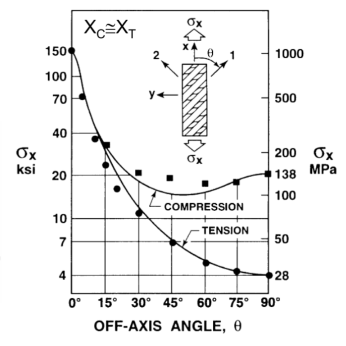
The results of the max stress theory are given in plot of σx with respect to the ply orientation [degree]. It is possible to observe some trends with respect to the material failure. The initial condition occurs when the structure is totally aligned with the stress field, which is in the x direction in this case. At this condition, the material exhibits its highest performance. If the structure is rotated in some degrees, the stress decreases. At the beginning, small values of θ, the failure will occur by shear. Rotating further occurs a quite deep drop down on σ_x. This is a region which the material can reach the condition |σ₁₂| ≥ S and fail by shear. When the structure is rotated up to 30°, another drop in σ_x is observed. However, this condition exhibits another trend, the matrix cracks in the transversal direction. Hence, the tensile stress still increases. The point of 30° also means the transition between shear and tension or compression. The trends of the curve are clearly different. This occurs due to the compression at the transverse direction, which is higher than the same at the longitudinal direction. Hence, it is more difficult to break the matrix and fiber in compression than in tension. It is also possible to notice that, the shear stress range is higher than the one for tension. The reason is that, the intersection between the shear and the failure occurs at a higher energy. Hence, when under compression, the stress range is quite small when the failure occurs at the fiber direction, is very large if the failure occurs in the fiber at the transverse direction and is smaller when the failure occurs in the matrix at the transverse direction. This graph illustrate the failure envelope predicted by the max stress theory. The final result of this one is that, the experimental data (black dots) are well described until about 30°. After this threshold, the approximation for compression is not so good as in shear one. In addition, the max shear stress envelope lost some points in the transition between shear and tension. For this reason, is not very accurate.

Tsai-Hill stress theory

The Tsai-Hill stress theory is part of the interactive approach. It is based in a polynomial series of second order equations which propose a non-linear combination of stresses. Actually, the Tsai-Hill is an adaptation of the Von-Mises theory in order to account the composite materials. In other words, the ones with strength anisotropy. However, the limitation of Tsai-Hill is that, to account strength asymmetry, it is necessary more information. Basically, the Tsai-Hill states that, the failure is prone to occur when the following equation is reached:

F(σ₂ – σ₃)² + G(σ₃ – σ₁)² + H(σ₁ – σ₂)² + 2(L•τ₂₃² + M•τ₁₃² + N•τ₁₂²) = 1

As can be seen, this relation includes terms that suggest that it is about a 3D laminate. It is a complete equation since it is based in Von-Mises. The main parameters are the properties of the material, which are given by the coefficients F, G, H, L, M and N. They are valid for anisotropic materials and usually are substituted by functions of 1/σ². Then it is possible to expand the equation for a single ply:

(G + H)σ₁² + (F + H)σ₂² + (F + G)σ₃² – 2[H•σ₁•σ₂ + F•σ₂•σ₃ + G•σ₁•σ₃]

+ 2[L•τ₂₃² + M•τ₁₃² + N•τ₁₂²] = 1

However, the assumptions made so far are considering only equally oriented plies. Hence, the terms τ₁₃, τ₂₃ and σ₃ can be considered zero. Therefore, only three components are really important, these are also called tests.

G + H = 1/x² ; F + H = 1/y² ; 2N = 1/S²

Then, substituting those components into the main equation, it is possible to obtain the failure index.

FI = (σ₁²/X²) – (σ₁•σ₂/X²) + (σ₂²/Y²) + (τ₁₂²/S²) = 1

This equation suggests that, a failure index equal 1 characterizes a material which is prone to fail. Interestingly, in the Tsai-Hill theory, FI accounts all the possible modes together in just one equation. Another step is to convert FI equation from the principal material direction to a function of the stress state, ply orientation and the material properties. This is done by substituting σ₁, σ₂ and τ₁₂ by their geometrical representation with respect to σ_x.

σ_x²•[(cos⁴θ /X²) + (sin⁴θ /Y²) + cos²θ•sin²θ•(1/S² – 1/X²)] = 1

Then, for each angle there is an allowable stress of the material, which is given by σ_x. The Tsai-Hill results are a σ_x-θ plot, which exhibits better results with respect to the max stress theory. Similarly to this ones, there are two curves respective to tension and compression stresses. In Tsai-Hill both curves are good approximations to the experimental data (black dots and squares).

The Tsai-Hill results also exhibits higher stresses in compression than in tension, which is the real behaviour. Hence, if the analysis occurs in tension, the curve is basically a continuous line. In the case of compressive loads, the curve is not so accurate as the tension ones, there is a small deviation from the experimental data. However, the Tsai-Hill criteria can be modified to account the asymmetry between tension and compression due to the material. This is given by several assumption for the material strength at x and y directions.

• X = X_t → σ₁ > 0
• X = X_c → σ₁ < 0
• Y = Y_t → σ₂ > 0
• Y = Y_c → σ₂ < 0
• X = X_t → σ₁σ₂ > 0
• X = X_c → σ₁σ₂ < 0

As can be seen, when σ1 and σ2 are lower than zero, it is necessary to change the value from tension to compression. In addition, the cross-terms (σ1σ2) also have similar assumptions. Hence they define when the material properties in x direction are equal to tension or compression strength. All those assumption are accounted in order to perform analysis with asymmetric lay-ups.

Hoffman criteria

The Hoffman criterial models the material in three dimensions, thus it also account for stress components at the thickness direction. This criteria is a sort of generalization of the Tsai-Hill ones. The reason is that, it takes into consideration the asymmetry in tension and compression strengths. In addition, it also considers the third direction. This means that, not only the in-plane strength values (Xt, Xc, Yt, Yc and Sxy) are accounted, but also the out-of-plane ones. These are the tension and the compression strength in thickness direction and the out-of-plane shear strength. The main equation of the Hoffman criteria is described as follows:

C₁(σ₂ – σ₃)² + C₂(σ₃ – σ₁)² + C₃(σ₁ – σ₂)² + C₄•σ₁ + C₅•σ2 + C₆•σ₃ + C₇•τ₂₃² + C₈•τ₁₃² + C₉•τ₁₂² = 1

As can be seen, the Hoffman criteria states nine constants which define nine strengths ate the orthotropic directions. These are X_t, X_c, Y_t, Y_c, Z_t, Z_c, S_xy, S_yz and S_zx. Actually, these constants also represent tests that should be done in order to characterize the material in all directions. These are described in Figure 8.

Some of those tests are difficult to measure, thus it is made assumptions. For instance, the test which involves Zt and Zc, mainly the test C6, are quite difficult to perform. The reason is that, a specimen for this test is very time consuming to build. Another assumption is regarding Syz and Sxy, because they are quite difficult to measure. Actually, there is no standard test for these parameters. Although only an interlaminar shear strength can deliver this result, it is not a reliable test. In this case, Syz and Sxy are usually considered approximately equal to Sxy. Since the analysis is focusing in equally oriented plies, the plane stress state is what really matters, thus it is possible to neglect the terms at the thickness direction (σ₃ = τ₁₃ = τ₂₃ = 0). Hence, the main equation is reduced to single ply one:

C₁•σ₂² + C₂•σ₁² + C₃(σ₁ – σ₂)² + C₄•σ₁ + C₅•σ₂ + C₉•τ₁₂² = 1

However, for composite plies some of these quantities are interconnected. Hence, it is possible to assume that Z_t = Y_t, Z_c = Y_c and S_xy = S. Those are substituted in the nine tests, then in the main equation. Hence, it is obtained the failure index for the Hoffman criteria.

FI = σ₁²/(X_t•X_c) + σ₂²/(Y_t•Y_c) + σ₁•σ₂/(X_t•X_c) + σ₁(Xt – Xc)/(Xt•Xc) + σ₂(Y_t – Y_c)/(Y_t•Y_c) + τ₁₂²/S² = 1

In this case, FI depends on both tensile and compressive strength. For this reason, the Hoffman criteria is more difficult to apply than the Tsai-Hill one. This has a failure index for compression and tension each. Another characteristic of the Hoffman failure index is the two linear terms into the equation. They yield a different orientation of the limit surface of the stress space (σ₁-σ₂-τ₁₂ plot) with respect to the same of the Tsai-Hill FI. Graphically, the axis of the ellipsoid stress space of Tsai-Hill is different from the Hoffman one. The practical effect is that, the Hoffman criteria is more flexible than Tsai-Hill one. As in the other criteria, FI = 1 means a region of the laminate which is prone to fail.

Tsai-Wu criteria

The Tsa-Wu criteria is described by a linear and a quadratic terms that define the direction of the stress. This theory is an extension of the Tsai-Hill one, thus it accounts also the strength at thickness direction. The main equation of the Tsai-Wu criteria is described below:

ƒ_i•σ_i + ƒ_ij•σ_i•σ_j = 1 ; i,j = 1, 2, 3, 4, 5, and 6

Similarly to the other theories, it is also made an assumption that the laminate is unidirectional. Hence, only the plane stress state is considered. This allows to neglect σ3, τ13 and τ23. Then Tsai-Wu definition becomes:

ƒ₁•σ₁ + ƒ₂•σ₂ + ƒ₆•τ12 + ƒ₁₁•σ₁² + ƒ₂₂•σ₂² + ƒ₆₆•τ₁₂² + 2ƒ₁₂•σ₁•σ₂ + 2ƒ₁₂•σ₁•τ₁₂ + 2ƒ₂₆•σ₂•τ₁₂ = 0

Another assumption regards the shear stresses, they revert the sign of the coefficient by reverting the reference system. Actually, this does not affect the ply, just the reference system. In practice, the problem is that, when the reference system is reverted, the failure index is not the same. It is necessary to keep it equal for positive and negatives. Since this is not what usually occurs, the term ƒ₆, ƒ₁₆ and ƒ₂₆ are kept zero in order to preserve invariances of the equation. Then, the Tsai-Wu criteria is updated:

FI = ƒ₁•σ₁ + ƒ₂•σ₂ + ƒ₁₁•σ₁² + ƒ₂₂•σ₂² + ƒ₆₆•τ₁₂² + 2ƒ₁₂•σ₁•σ₂ = 1

Now, it is possible to notice that, Tsai-Wu and Hoffman have very similar failure indexes. Both have coefficients which are dependent on test and are related to material properties. This coefficients are described below:

As can be seen, those are given by different tests, where ƒ₁ and ƒ₁₁ are the longitudinal tension and compression tests. The transverse tension and compression test are given by ƒ₂ and ƒ₂₂, respectively. In addition, the shear tests are accounted by ƒ₆₆. There is also the interaction coefficient, represented by ƒ₁₂. Usually, it depends on tension and compression tests at both directions. In addition, it is the test that differentiate the Tsai-Wu from the Hoffman criteria. In other words, ƒ₁₂ is basically the product of σ₁ and σ₂. In the Tsai-Hil criteria, this product is multiplied by 1/Xt, thus a very similar parameter. The Tsai-Wu and Tsai-Hill criteria exhibit almost equal results, while the Hoffman criteria is a mid term between these. Usually, the Tsai-Hill is more adopted, because the interaction coefficient has a higher weight in the extreme angles.

References

• Mallick, P.K. Fiber-Reinforced Composite: materials, manufacturing and design. Edition 3, CRC Press, 2008.
• This article was also based on the lecture notes written by the author during the Design for Composite Structure of Racing Car lectures at Unimore.