In the previous articles (read them here and here) it was described the formulation development in order to get the CLT equation. Through this, it was noticed the relation between load and deformations, membrane loads and strains and the effects of the coupling. In this article the coupling effect will be qualitatively explained and the CLT limitations will be exposed. At the end, a brief explanation of the finite element methods for CLT is done.

Effects and importance of the coupling

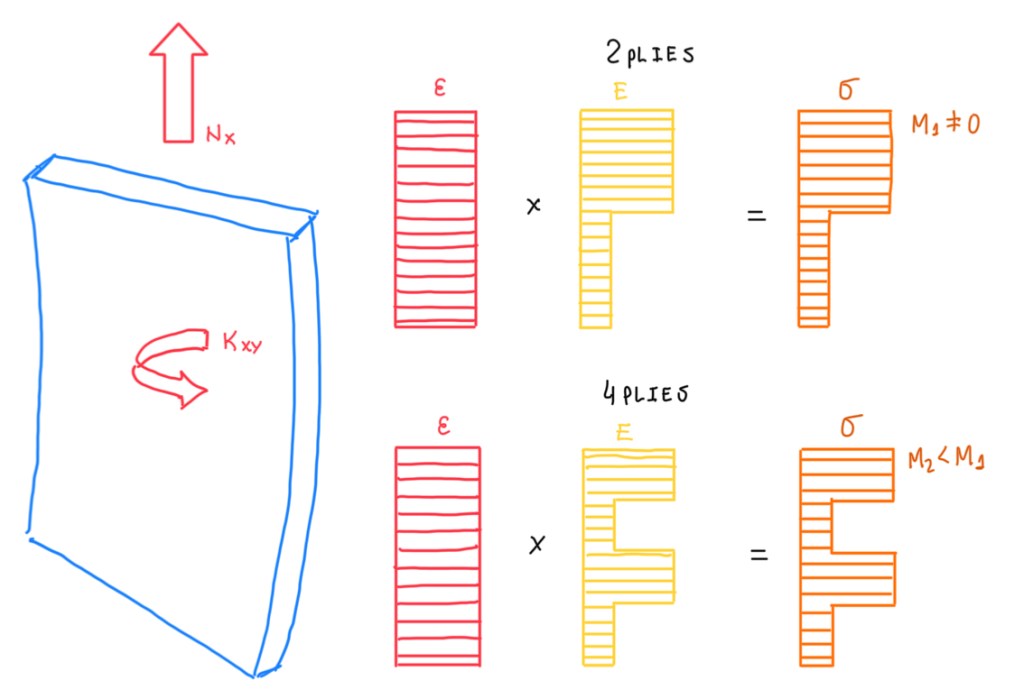
For the designation of coupling, for instance, the membrane strain, torsional or twisted curvature, its reason is qualitatively explained in Figure 1. For example, the membrane strain non-symmetric properties and bending moments means that, something occurs in terms of bending or twisting. Figure 1 illustrates two different cases, one with two plies and another with four plies. In this case, it is possible to notice that, the asymmetry of the resultant stress distribution is lower than the previous case. This qualitatively means that, if the layout has more plies, even if these are not symmetric, the coupling will be lower and lower, as long it is increased the number of plies. Hence, as higher the number of plies, the lower will be the effects of coupling. A larger number of plies null the coupling independently if they are symmetric or not.

Stresses in the k-th ply

The dimensional case means, passing from fibers to plies, from plies to laminate and, in some cases, from plies to fibers and from laminate to plies. The objective is to understand that once known the deformations on the laminate, it is possible to know the deformations on the plies, which is dependent on the laminate mid plane from the ply times the curvature. The distance from the mid plane is taken as the average of the distances of ply interface ones. If there is strain in each ply, by the stiffness matrix of each ply, it is possible to calculate the stress.

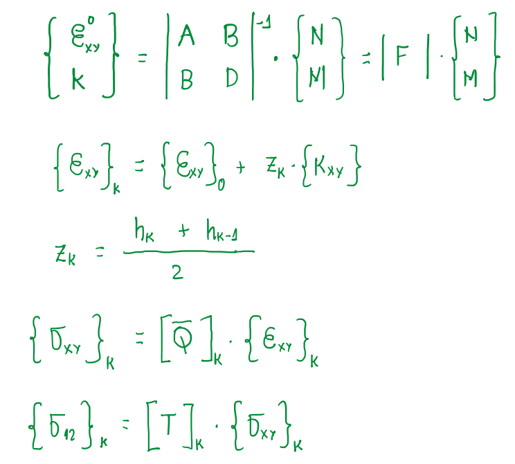
To understand the stresses on the principal material direction, introduced by the calculation of the redundancy of the ply saturation, it is just necessary to make the transformation of the stresses into the principal material. Obviously, it is possible to notice that, such calculation are performed by proper devices, but it is important to understand the path of these.

Limitations of classical lamination theory

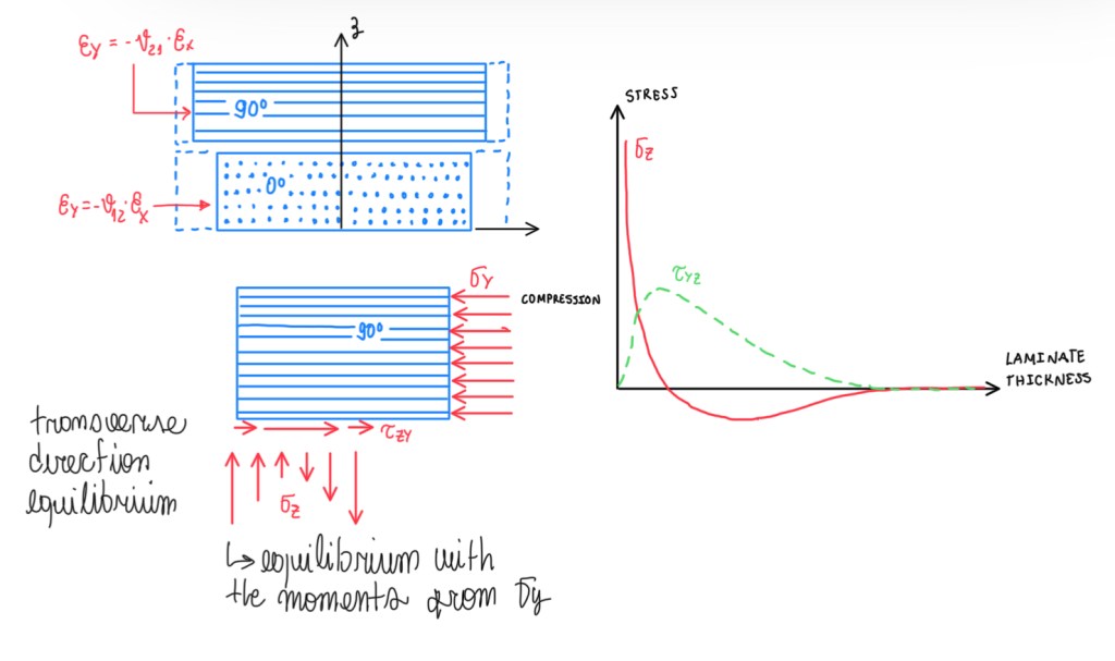
The limitation of the classical lamination theory is that, it does not account the Poisson mismatch between the plies. For instance, in the case of plies oriented at 0º (Figure 3), they are also oriented out-of-plane. Another limitation is the transverse shrinkage of the plies of the loads applied at 0º and 90º, which are ε_y = -ν₁₂•ε_x and ε_y = -ν₂₁•ε_x, respectively. The 90º transverse shrinkage is much lower than 0º one, because in this case there are fibers which prevent the contraction. Hence, these plies are together and there are some stresses that compensates this mismatch. These stresses are shear ones, but if these occur on the direction seen in Figure 3, it is necessary to compensate that with a compression stress σ_y. However, this generates a bending around the corner, this is compensated by the stress distribution along σ_z. Specially this value on the interface τ_zy, have a qualitative trend which is characterized by peak value of the shear stress, the dotted line (Figure 3), and the asymptotic value of the transverse σ_z. This problem can be better explained understanding these two plies separately. In this case, they are inverted, thus they are only suffering a different compression. Once they are put together, these will carry the same deformation, which means that one has to expand and the other has to shrink. Hence, there will be forces addressed at the limit of the stress and, at the interface, the stresses are characterized by the direction with respect to mounting ply, because they have to shrink the ply. This means that in terms of balance, there are compressive stresses transverse to the ply. Regarding the equilibrium, certainly there is in terms of the transverse direction. Hence, for the moment generated (Figure 3), there is some equilibrium. The case seen in Figure 3 illustrates that, about the corner of the ply, there is a moment. In this case, it is necessary another stress distribution, which is σ_z, to balance the one represented by σ_y. In other words, the moment generated by σ_y distribution is balanced by the same generated due to σ_z. Bottom line, the distribution of the stresses are much more complex than the one that is modelled. These are stresses that can be modelled by maths and FEA.

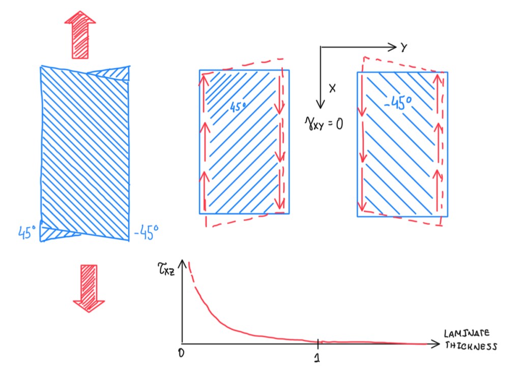
The stresses due to shear deformation mismatch, also called shear disagreement, are illustrated by Figure 4. In this case, the plies are at -45º and 45º, because each single ply are subjected to a membrane load that deforms both in tension and in shear due to the fact that, the fibers are off-axis. The fact that the angles are 90º to the one with respect to each other means that, the shear deformation will be mismatched between the plies. For the deformation equalises, the balanced lay-up has an extension deformation. In other words, there is no shear deformation on the overall -45º/45º composite. Actually, this means that there are shear stresses at the interface, which brings back the two plies to a consistent deformation. In addition, the stresses have a qualitative trend that suggests a theoretic infinite value close to the sides. In other words, these can reach very high values close to the sides and potentially damage the laminate at the interface. Hence, this is a reason why it is advisable to not have very large angles between one ply, the following and the previous one, because it is generated a larger shear mismatch. The larger the angle, the larger the shear mismatch. Those are values of stresses that can not be calculated by the classical lamination theory. Actually, those are calculated by sophisticated algorithms on the finite element method (FEM).

Through-the-thickness and the interlaminar shear evaluation

The assumption that the laminate is done by a sequence of plies, which are subjected to a in-plane stresses characterised just by σ_x, σ_y and τ_xy in each ply, is addressed to thin laminates. If the laminate is thicker, then the transverse shear stress will be higher. Similar as beams, as thicker they are, higher will be the transverse shear stress with respect to the bending stresses. Hence, for the thick laminates, the assumption of negligible interlaminar shear stresses may not be true. In addition, in the case of an isotropic material and if that assumption is considered, this is quite similar to have a beam which its thickness to length ratio is too low. In this case, the shear modulus is comparable to elastic modulus (G ≅ E), thus G < E for isotropic materials, which typical for metals it is about 2.3. It is more than one third of the elastic module.

E = 2G•(1 + µ)

In the case of components, the value of G₁₃, which is most often also a representation of G₂₃, is much lower than the value of E₁. This means that, a small shear on the transverse direction, even at a small shear load, will result in a high shear strain, because the value of the module is low. Therefore, it is necessary to account the presence of the transverse shear stresses and deformations in order to have a proper representation of the stress and strain in a composite. This is the reason why there is a method called, first shear deformation theory, which is an enhancement of CLT, that considers the presence of the transverse shear ω_x and ω_y, which are balanced by the shear stresses, τ_yz and τ_xz. In other words, a summation of the shear stress of each ply, for all plies.

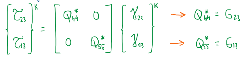
There are some steps for finding the relation between the transverse shear stress and the transverse shear strain for each ply. Where these properties are nothing else than those elastic moduli described in Figure 5. Hence, there is no G₁₂, in this case it is the elastic modulus in-plane G₁₃, the elastic modulus out-of-plane is G₂₃.

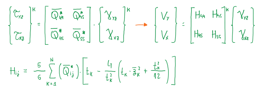
Hence, there are some steps to get the representation of the relationship between shear forces, loads and deformations through a matrix, which are characterized by terms that depend on the shear stiffness matrix of the ply summed over a number of plies times a function of the thickness.

Basics of finite element analysis for laminates

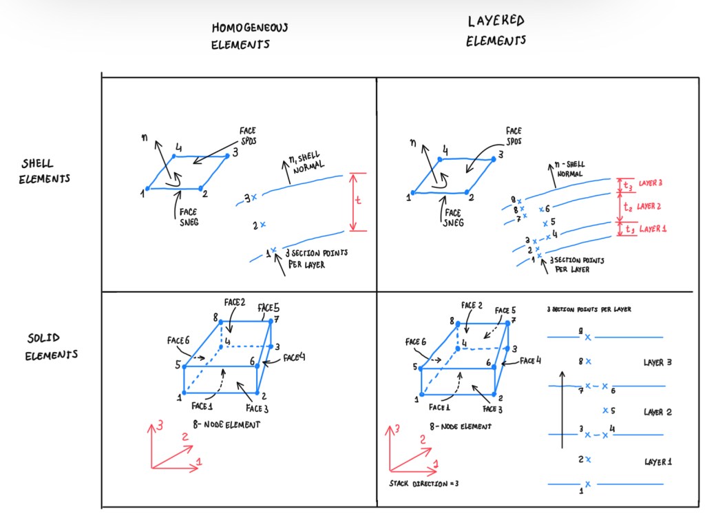
The finite element analysis for laminates has several choices. Figure 7 illustrates some perspectives. For instance, shell and solid elements can be chosen as well the configurations homogeneous and layered. The homogeneous elements mean that each element is defined equivalently to the orthotropic ply. The layered element is a configuration which each element has a lay-up that composes the element. For instance, there is a command which is called, composite lay-up, which the orientation of each ply composes the section of a shell or the section of a hollow. Obviously, each ply refers to a determined material, which its properties are given in the principal material direction. Hence, given a lay-up, the software calculates the stiffness matrix of the ply, or the same of the laminate. When using different types, for instance, if it is requested to perform a first attempt analysis of a body where there is no very critical points, like holes, sharp curvatures, corners and edges, it can be used shell elements. These are computationally light and simple. If it is found a material which is homogenous with respect to the thickness and orthotropic, thus it should be defined orthotropic equivalent ply properties of the laminate. The reason is that, the section which is attached to a square element defines the properties of the laminate. It is possible to use solid elements with more elements through the thickness as possible and to use more elements for each ply, if these are explicitly modelled. The material used is different for each ply. In this case, it is useful to study interlaminar shear stresses across the interfaces.

Layered elements

The use of layered elements is similar to homogenous elements. The difference is that, instead inputing orthotropic properties, it is configured the lay-up and defined a material according to its orthotropic properties in its principal material direction.

Continuum shell elements

Continuum shell looks like a solid element, thus it is possible to mesh a three dimensional geometry with a solid hexahedron. However, in this case instead, it is extracted the mid-surface and the mesh with elements, which its kinematic and constitutive behaviour is like a conventional shell element. Hence, it is more convenient for mesh purposes. Since the solid elements have just displacements and degrees of freedom, the continuum shell elements have displacements and nodes. From those it is calculated the rotation corresponding to thick tissue nodes at the midplane of the element as it was a shell. Hence, below this membrane there is a shell, where the rotations are calculated by the nodes at the displacement. In this case, it brings infinite membrane strain and large rotations up to 10%, thus solid elements are preferable.

References

• P.K. Mallick, Fiber-Reinforced Composites: materials, manufacturing and design – 3° Ed., CRC Press, 2008.