Another important topic which is improved during the motorsport design process is the noise. Usually, these are concentrated in high performance vehicles, but the processes used are derived from the racing field.

Wind noise in road vehicles

The wind noise simulation is commonly performed in road cars. There are three major sources of wind noises in road cars, the wind rush, the leak and the cavity noises.

Wind rush noise

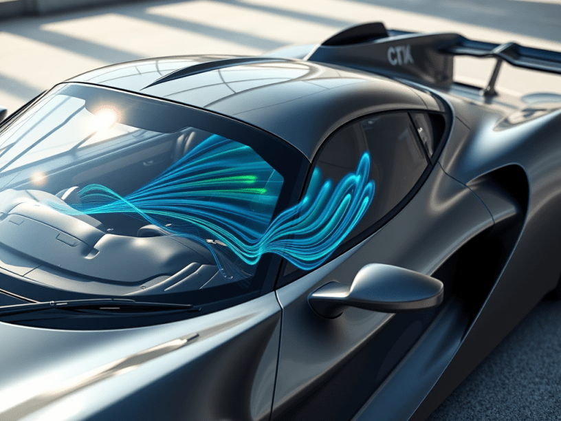
The wind rush noise is produced by the interaction between the free stream and the vehicle body. A common example of this kind of noise is the A-pillar (Figure 1). It creates a lot of very coherent vortices that impact the mirror. Since these are very close to the passengers, they create a very uncomfortable noise. In addition, this area is critical, because it is part of the vehicle architecture and has an important effect on the structure. Hence, it is important to analyze this kind of phenomena in the very first stages of the design process, in order to engineer ways to reduce as much wind noise as possible without a too reduced pillar. If in the latest part of this process this issue is detected, it is very difficult to fix it. The reason is that the A-pillar is constrained by structural calculation and putting fins can result in unexpected damage. Hence, it is crucial to define the considerations about the wind rush noise at the beginning of the design process.

Leak noise

The leak noise is the whistle that is generated due to the flow over small gaps. The leak noise is very complex, because it is typically found in the later stages of the process. Hence this is something that can not be improved at the beginning, instead it can be simulated at the end of the process. The reason is that it requires high fidelity geometries, which is only available when the process is at the final stages.

Cavity noise

The cavity noise, like the wind rush one, can be predicted in the beginning. The buffering effect is what starts the cavity noise, it is a low frequency and high sound pressure noise which occurs in a cavity. For instance, the noise due to the air flow through the trail of the sun roof.

Acoustics

Considering these phenomena in terms of simulation, it should be interesting to understand what is acoustic and what is noise. The sound is a pressure wave propagation that can be reflected, refracted, attenuated and undergo convection by the medium and, not less important, by the surfaces. The medium property affects the sound with the state equation. In other words, the relation between density, pressure and temperature is what determines the sound speed.

Aero acoustic index

SPL = 20∙log₁₀(P’_rms/P_ref) ; P_ref = 2∙10^-5 N/m² (air)

In terms of acoustics, the main index is the sound pressure level (SPL), it is expressed in decibel (dB), which is defined as the ratio between the root mean square (RMS) of the pressure fluctuation and the reference pressure, this one is the pressure threshold of the human hearing at 1 kHz. If a noise has its index computed, it will be possible to see as a function of the noise frequency, the curve of SPL, which is representing how noisy the signal is at different frequencies. Another index is a more global one. The equivalent sound pressure level L_eq is an indicator of how noisy the full signal is. This is given by the logarithmic of the SPL signal.

L_eq = 10∙log(∑_i=1^N 10^SPL_i/10)

The sound pressure level (SPL) is given in dB, but this is a global measure. Its meaning is not related to human hearing. This is important since cars are developed according to human comfort and ears perception. Hence, the dependency of the human threshold must be re-introduced.

The SPL signal is weighted by a specific curve, this is the A-frequency weighting curve, which is a very well known weighting function available in the industry by the international standards. It is based on how the human ear is able to perceive different sounds. Figure 3 illustrates those functions, the A-curve (blue), as a function of frequency, this curve suggests that from 1 kHz to 10 kHz, the human ears have a perception of sound as it is, but also amplified. Hence, if a sound lies between 1 kHz and 10 kHz, this would be an annoying one. When the disturbance sound is below 1 kHz, the human ear is able to reduce the dB perceptivity. Therefore, the A-curve is always used to weight the SPL definition and have a base curve in terms of acoustics. There are other kinds of curves, like the D-frequency weighting for example, which is used for aircraft noises.

Aero acoustic models

The acoustic models vary between them according to how the acoustic is quantified and simulated.

Computational aero acoustics CAA

This model is based on the solver of the pressure fluctuation directly into the CFD environment. Hence, there is the CFD solution, the transient CFD simulation and the material characterization. This model requires a huge computation, but it is a complete calculation. The good point in acoustic simulations is the no requisition of a high concern about the turbulence scales. The attention should be dedicated to the frequency solution in terms of noise generation. Hence, the mesh resolution will be finer with respect to the transient external aerodynamic one. It is not just a matter of turbulence, instead it is also a matter of which frequency is being used to solve the simulation. The computational aero acoustics model is very complete and accurate for noise generation, but it is too time consuming. This is not the sort of time that such simulation requires to have a picture of what is happening in terms of noise generation. Indeed, with a lot of time is easier to go with this simplified model and try to change the macro-layout and observe how the sources of noise are behaving, instead of waiting for weeks to have a complete simulation. Therefore, CAA includes all the effects, but requires an analysis of a transient compressible simulation.

Coupled CFD/BEM

Since CAA is the most complete model, there are some simplifications. One of them is the coupling with different codes, more precisely, specialized acoustic ones, boundary element methods (BEM) and hybrid zonal methods. These use CFD to track the sources, then another software is collecting these from the high fidelity CFD simulations and solving the wake propagation.

Acoustic analogy

The acoustic analogy modeling is a quite similar model to the coupled CFD/BEM. This is used by CFD to track the sources and the analytical solution to propagate the sound.

Steady RANS / Turbulence correlations

The steady RANS based noise source modeling simulation is not transient, instead the runs are steady and it is used empirical correlations to estimate the sources. However, there is no concern about how the sound is propagated. It is only analyzed how well the sources are. In other words, if the options are reducing or increasing the sources of noise.

Broadband noise models

The broadband noise models are the formal name of the steady RANS that are able to detect the sources of noise. In this model it is not possible to evaluate the sound that the receivers are hearing, but it is possible to analyze the sources since it is just post-processing.

Models summary

To summarize those models, their limitations and features are illustrated at Figure 4. The model features are the default modelling CAA, the computational acoustics coupled with another softwares (Coupled CFD/BEM), acoustic analogies and turbulence correlations. Apart for this one, these all need a transient CFD, which is also interesting from the engineering point of view. The requirement of a compressible solution is not necessary in all of them. The reflection and the scattering are another key points that the engineer must remember when choosing the model.

Examples of model applications

Figure 5 illustrates an example of a computation aero acoustics model applied for a road car side mirror. This is the studying of the noise generated by the coherent structures that comes from the side mirrors.

Figure 6 illustrates the same analysis performed on the A-pillar. These two basically are the aero acoustics analysis, in other words, the analysis of the sound generation on the windscreen area. The A-pillar and the side mirror are the most critical parts in terms of noise generation. In addition, the VSR of the A-pillar suggests that dB level has a very good correlation. CAA is performed in convertible cars, because the flow detaches from the windscreen and imparts inside the cockpit area. This creates a huge noise. If the results of the structure are very coherent, it induces a phenomena called buffeting. To avoid this it is required to either test some options with the broadband noise or test the final ones with the computation acoustics to verify how it is behaving in terms of the velocity magnitude, the power spectrum, the sound pressure level at the area of the air. An important trick for acoustic simulations is to not focus on the sound generating area, instead, concentrate on the receiver area, where the driver and the passenger are. In cases of homologation, this is important to decide where to put the microphones, thus the sound could be huge everywhere, but lower where the microphones are.

Fluid-structure interaction problem

The fluid-structure interaction is one example of Multiphysics, which links laws from CFD, the aero and the displacement from the structural deformation. The fluid structure method is crucial such that there are areas from the more passive one to the more active one. The passive area is the one that it is required to check as a secondary effect, while the active area is the one that the secondary effect is to carry the user to extract performance. Safety (Figure 7) guarantees the structural integrity of the area. During a lap there are high loads and velocities that require a proper structural integrity. The homologation (Figure 7) is important, because there are many regulations and these have constraints regarding the structural deformation. The performance (Figure 7) loss is the first secondary effect. Deformation cycles can cause gradual degradation of the structure. For example, when suspensions are performing deformation during the use, the continuous cycles result in different wheel positions as camber variation due to components degradation. Hence, the car starts an outing with a predefined camber, but finishes it with a considerably out of range value. The performance development deals with the aerodynamic development guiding structural deformation.

To achieve this kind of design it is required to be totally confident about the FSI approach. This is performed according to the application. For instance, in road cars the structural integrity is verified according to how the deformation is performed during the representation cycle. In the first iteration this is always an over prediction of the deformation. Hence, if it is required to check the structural integrity in some mountings, it is possible to stop the process in the iteration zero and check if the structure is okay. The iteration zero is the nodes distribution when it matches the structure of the CFD model, this is checked to verify which are the deformations. Forced iteration is when the structure is under certain deformation, this changes the shapes, thus the loads. Hence, with this displacement it is necessary to update the CFD simulation, solve the loads again, put the new loads on the structure again, and re-check the new displacement. There are two approaches to solve FSI, the classic method and the two-way coupled one.

Classic method

The classic model approach is based on finding the structural point of view (Figure 9). The structural theory allows us to know that every displacement can be a linear combination of the eigen-vectors and eigen-values. Hence, there is a model, its eigenvectors and eigenvalues are extracted and its combination, if it is a linear displacement, it can deliver which are the displacements of the structure. This is a strong concept, because if it is put the eigenvectors and eigenvalues computed for a structural model into the CFD solver, the result is a CFD model aero-elastic. In other words, a CFD model which is able to predict loads. The eigenvectors and eigenvalues are mapped into the CFD solver as well. Hence, once the load distribution is calculated, the structural equation defines the thickness and the modal displacements. The thickness includes the eigenvectors, thus if the equilibrium is solved, it is possible to compute directly into the CFD solver, which is the displacement of the structure. Therefore, regarding the non-deformed geometry and the structural solver, it is put the modes and frequency into the aero solver, it is computed for loads, it is solved the equilibrium between stiffness of the structure and loads from CFD and automatically it is possible to compute the displacement into the CFD software. If it was able to deform the mesh, this is deformed and goes back to the beginning of the loop (Figure 9). Hence, it is closed in the FSI loop with just one solver. The mesh can be surface or volume ones, it depends on the case.

Some components have a strong displacement, while others have a very small range. For example, for wings, 10 mm is a common number since these can not deflect too much, because it is restricted by rules or, in the case of the front wing, there are limits due to the stall. The classic approach is a good one, because it allows inputs of extra models and frequencies from the structure. Typically, for wings as the one at Figure 10, it is requested just 4 – 5 modes. It is not so expensive, in terms of time. This can be added to the CFD solver and this one can run the FSI solver inside the CFD solver. The problem with the FSI classic method is that it is based on a linear behavior of the displacement and on a model. A wing, as the one at Figure 10, has about 25 profiles, which is not so interesting for a model based on modes. In this case, it is necessary to have 25 modes, at least, to picture correctly the displacement. This is a very nice method, but it could not be the solution for interconnected areas. For instance, the F1 car has a link between the dynamics of the car and the area of the flat floor and the rear wheel, which are very interconnected to the body.

Two-way coupled method

The two-way coupled approach is an iterative process that looks for convergence of both displacement and load. Hence, the iterations go from loads to displacements and from displacements to loads until the structure and the aerodynamics are stable. This is not such a long process, it requires typically 4 – 5 iterations at maximum to reach the converged solution since it is a static deformation. This method is based on CFD and FEA workflow, the best practices of both methods. Since there are total processes and meshes, it is required a highly precise mapping of the loads of the unmeshed model and highly precise mapping of the displacements that are found on the FEA model. The displacement should be updated by the CFD meshing in some way. It is possible to activate both surface and volume meshes and it uses the complete workflow laws, thus this method requires a high computational effort and should be guided by a kind of externally orchestrator, which is activating different tasks with respect to a complete cycle.

References

• This article was based on the lecture notes written during the Industrial Aerodynamics lectures attend at Dallara Academy.