Circulation can be defined as a measure of the combined strength of all vortex lines passing through a surface S. It is usually given by:
Γ = ∳cƒ∙dl = ∫s curlƒ∙n∙dS
where ƒ is the continuous field. Applying the Stokes theorem with continuous partial derivative on the surface S, the result is the integration of the curl of the continuous field and the normal vector about the surface area. Actually, circulation is a tool used by Frederic Lanchester, Wilhelm Kutta and Nikolai Joukowski which, defines that a closed curve C immersed in a flow field can exhibit fluid elements moving in a circle within the flow field.
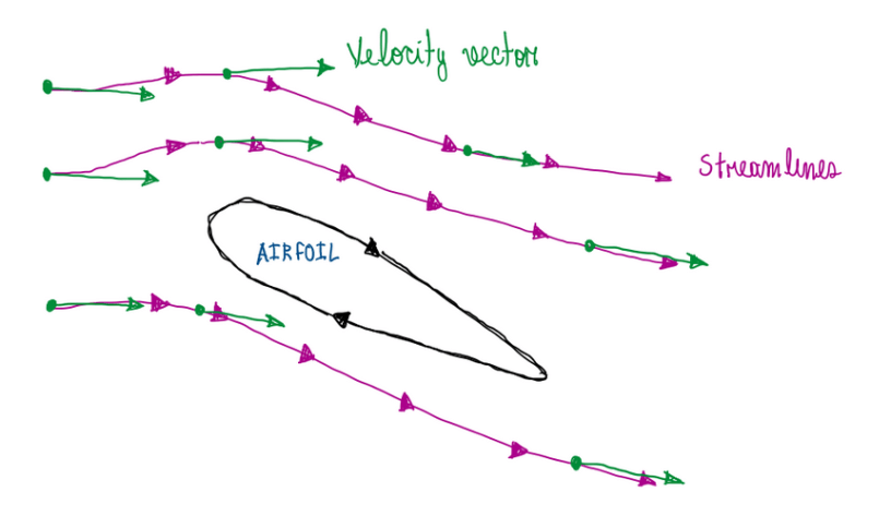
However, in aerodynamics, circulation term may not mean a circular flow of particles inside the flow field. For instance, an airfoil that is generating lift as illustrated by Figure 2.
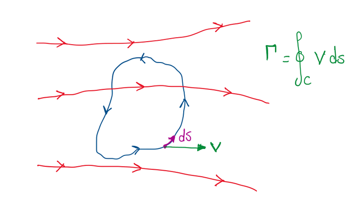
The circulation exhibited around a closed curve that encloses the airfoil will be infinite, despite the fact that fluid elements are not executing circular movements around the airfoil. Another interesting point about circulation is its relation with vorticity. For this case it is interesting to assume a surface inside the flow field as seen in Figure 3.
This is an open surface bounded by the closed curve C, thus the circulation about a curve C is equal to the vorticity integrated over any surface bounded by C. This can be described by the following equation:
Γ = ∳c V∙dS = – ∫∫s (∇×V)dS
The result of this equation is, when the flow is irrotational everywhere within the contour of integration (∇×V = 0), circulation is zero, Γ = 0. If the curve C is shrunken until a point that it admits an infinitesimal size, the previous equation can be updated to:
dΓ = -(∇×V)dS = -(∇×V)∙n∙dS → (∇×V)∙n = – (dΓ/dS)
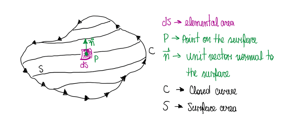
Where ds is the infinitesimal area enclosed by the infinitesimal curve C, this can be illustrated by Figure 4.
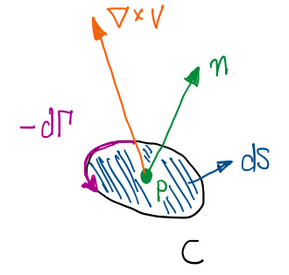
Hence, at point P inside a flow, the component of vorticity normal to ds is equal to the negative value of the circulation per unit area, where the circulation is occurring around a boundary with surface dS. Therefore, it is understood that circulation is a flow of fluid particles about a surface. It can be circular or not. In addition, the vorticity is basically the circulation per unit area.
Elliptical circulation distribution
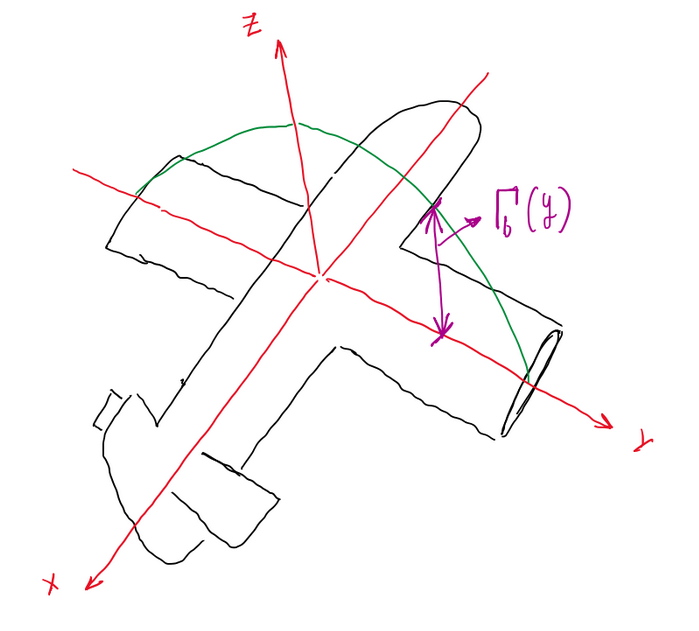
Since a brief review about circulation is performed, it is possible make some comments about the elliptical circulation distribution. The circulation in a wing with span wise b is defined as maximum at the middle of the wing as illustrated by Figure 5.
Hence, it is possible to write that circulation at y = 0 is:
Γb(y = 0) = Γb,max = Γ0
Since the equation of an ellipsis is already known, it is possible to adapt it to describe the circulation about a wing.
(Γ(y)/Γ0)² + (y/(b/2))² = 1
Where Γ0 and b/2 are the semi-axis of ellipsis while Γ(y) and y are its variables. If Γ(y) is placed as reference, this equation is updated to:
Γ(y) = Γ0√[1 – (2y/b)²]
Applying the Kutta-Joukowsky theory per section, it will be obtained that also the lift (L’) will be elliptical in its distribution. In addition, according to the line theory, it is possible to find a relationship between the trailing vorticity γt and circulation Γb(y).
γt = dΓb(y)/dy = 4Γ0∙y/[b²√1-(2y/b)²]
Figure 6 illustrates the equation above in a 2D graph.
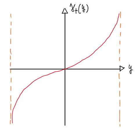
This description would not be completely physical, because it implies in an infinite circulation distribution at wing edges. Ir is this vorticity distribution at axial direction that creates an uniform downwash velocity, which is given by:
ω = – Γ0/b
For elliptical lift distribution, downwash is constant over the wing span. Since the elliptical distribution is already defined, it is possible to evaluate the consequences of this one. The induced angle of attack is given by:
αi = CL/πAR ; αi ≈ CD,i/CL → CD,i = CL²/πAR
It is important to remember that the aspect ratio is given by:
AR = b²/s = b²/c
Through those equations it is possible to visualize the geometrical impact of the wing on the induced drag and the lift coefficients.
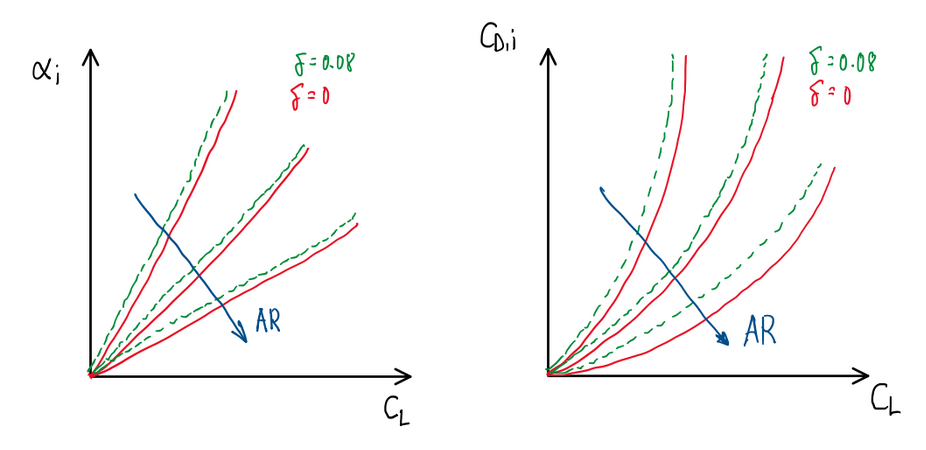
As can be seen, as soon AR decreases, which means a bigger chord or surface area, and for the same CL, the induced angle of attack produced is reduced. Consequently, the induced drag coefficient CD,i is also lower. In case of non-elliptical wings, the results are even worse.
Chord distribution for elliptical wings
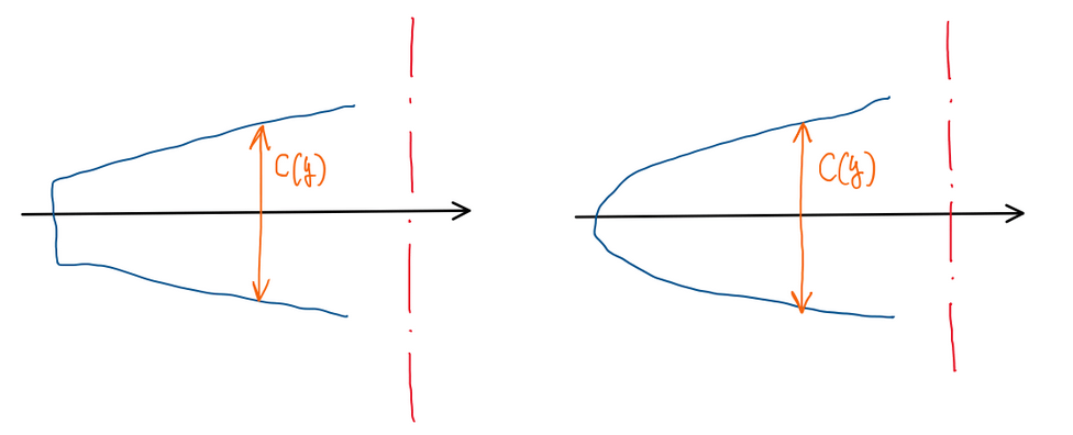
The chord distribution determines the wing geometry. Actually, it is possible to determine the distribution of the chord corresponding to the circulation and lift distribution of an elliptical wing. This is a specific chord distribution, that correspond to the circulation and lift distribution with elliptical characteristics. Hence, applying the Kutta-Joukowskhy theorem, it is given the following equation for lift.
L’ = ρ∙U∞∙Γb(y)∙cos(αi)
From the thin airfoil theory, it is possible to update this equation to:
L’ = 2π(αeff – α0)∙c(y)∙q∞
To simplify, it is interesting to assume that α, α0 and αi is not a function of y, this means that there is no aerodynamic twist nor geometrical twist. The only y dependence is the circulation distribution, thus it is possible to write:
L’ = 2π(α – αi – α0)∙c(y)∙q∞
Hence, an elliptical chord c(y) provides a lower induced drag. A non-elliptical wing exhibit a worst behavior relative to an elliptical one, but it is not enough to justify the complexity of an elliptical wing.
References
- Anderson, J. Fundamentals of Aerodynamics. McGrawHill Education, Ed. 6, New York, 2017;
- Stalio, Enrico. Aerodynamics. October, 2021;
- http://www.aerodinamica.unimore.it
