
The main objective of the micro-mechanics is the calculation of the material properties by the knowledge of its volume fractions. Certainly, this is a prediction, but it is widely accepted due to its reasonable accuracy and precision. This article proposes a brief discussion of the formulations of these predictions and the models used for that.
Viscoelastic Models for the prediction of the properties
The hypothesis that are behind the usual models are homogeneity, orthotropy, linearity of the constitutive response and the residual stresses. The homogeneity defines that, the properties are evenly distributed over the material. It is not considered a point-to-point variation of the properties in order to simplify the calculations. The orthotropy is a hypothesis that means the existence of different planes of symmetry into the material and the definition of four independent elastic constants. For instance, in the case of a simple isotropic materials, as metals in general, there are just two independent elastic constants, the Young’s modulus and the Poisson’s ratio. The linearity of constitutive response is assumed. It is about 2 for fibers, which are inherently brittle, but also for thermosets or epoxy matrices. These do not exhibit a plastic or non-linear response. The residual stresses may come from the heterogeneity and thermal expansion mismatch, which do not modify the properties that will be estimated, as stiffness and macroscopic strain homogeneity. The thermal expansion mismatch means that, when there are several constituents in a material, generally each of them have a different coefficient of thermal expansion. Hence, the composite material is heated or cooled down, the different constituents will try to expand or to contract at different rate from each other. Since the expansion and the contraction of the whole material is the same, then some stresses will occur in order to keep the material continuity and compensate the thermal expansion mismatch of the constituents. However, this does not affect the behaviour that is estimated. The first equations that should be considered involves volumes and weight fractions and the density of the material.
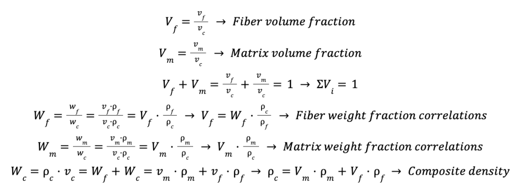
The volume fraction, by definition is the volume of the fiber or the matrix divided by the volume of the whole material. Hence, the sum of the volume fraction should be equal to the unity. The weight fraction can be more easily measured, since the volume fraction often depends on the process used for it. For instance, composite laminates can be made by a vacuum bag process. In this case, there is the possibility to insert a foil, which can be perfurated or not in order to let the epoxy to flow out from the laminate, or to keep it into the laminate. This changes the final volume fraction of the fiber and the matrix. In the case of the weight fraction, the matrix or the fiber can be measured before to assembly them into a pre-preg, for instance. The definition of the weight fraction is the ratio between the weight of fibers or matrices by the weight of the whole material. Figure 1 also illustrates that the weight and the volume fraction can be correlated. The weight can also be defined by the density times the volume, thus it is possible to put the volume fraction into the weight one. Hence, the weight fraction definition can be also given by the product between the volume fraction and the density one. This definition is also useful to estimate the density of the composite given the volume fraction and the density of the fibers and the matrix. Since the total weight of the composite is the sum of the weight of the phases, fibers and matrix, if the weight is written as density times volume, then it is possible to find the definition of the composite density. This is the sum of the product of the volume fraction by the density of the fibers and the matrix. This is called, the rule of the mixtures. It is given by two constituents, that are mixed-up and the property of the mixture is the weighted property of the constituents.
Young’s modulus with randomly distributed inclusions

Another important property to measure are the mechanical ones, an example of these is the Young’s modulus. Considering a composite with randomly distributed inclusions, the hypothesis that lies beneath this model is that fiber and matrix exhibit purely elastic strains (εf, εm). The applied stress σ is shared as σf and σm for fibers and matrices, respectively. The fiber volume fraction is given by Vf and Vm and the elastic modulus of the constituents (Young’s modulus) are given by Ef and Em, for fiber and matrix, respectively. The inclusion shape is not considered in the model, since it is assumed to have a stochastic distribution in random orientation. Hence, it does not affect the result locally. Another hypothesis is the perfect adhesion between fiber and matrix, thus there are no additional stiffness or compliance in the interface between fiber and matrix.
Voigt model (upper bound)
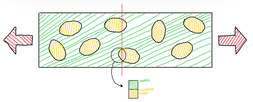

For random oriented inclusions, it is defined two bounds, upper and lower ones. Depending on the orientation of the plane that cuts the composite, the upper bound is found by the plane orthogonal to the forces applied on the composite. If this is cut as seen in Figure 3, then it is possible to spot that at the interface between the matrix and the inclusion working in parallel with respect to the loads. This means that, they are experiencing the same strain, which are equal to the global strain of the composite. This is the assumption made by the Voigt model (Navarro,2017). Therefore, to evaluate the Young’s modulus of the composite, which by definition of a linear elastic behaviour is just the stress divided by the strain, it is possible to write the stress as the force divided by the section of the fibers and the same for the matrix. This means that, it is obtained the ratios Af/A and Am/A, that are basically the volume fractions of fibers and matrices. The reason behind the area fraction becomes the volume fraction is the assumption of an unit thickness and unit length. Hence, the volume is essentially independent on the third dimension. Moreover, the strain is the same for the fiber and the matrix, thus it is possible to substitute either εf and εm by ε. In the end of the calculation, it is possible to observe that the upper bound modulus is just the rule of the mixtures but applied to the Young’s modulus of the material. It is also possible to notice that, this rule is quite similar to the equation of two springs in parallel. This defines that, the total stiffness is the sum of the stiffness of the two springs.
Reuss model (lower bound)


When the composite is cut in a plane parallel to the applying load, this is called the Reuss model. In this case, considering the two faces between the inclusions where the load is transmitted, they are working in series. Hence, matrix and inclusion are working in series with respect to the load. This means that, the strain will not be the same for fibers and matrix, but the stress will be the same for them. Hence, applying the same procedure of the Voigt model to define the Young’s modulus, the arrange will be different. In the Reuss model, the strain is multiplied and divided by the length l, which is the length of the composite. However, the product of the strain by the length l is basically the deformation of the composite. Then this can be assumed as the sum of the deformation of the fiber and the matrix. Assuming that lf and lm are general parameters that define how matrix and fibers are deformed into the composite, it is possible to consider the volume fractions. From the point of view of modelling, this assumption is correct, there are fibers and matrix deformations which contribute for the total deformation. Then, the equation seen in Figure 4 is multiplied and divided by the section area (A/A). Hence, A•lm and A•lf will be the volume of the matrix and the fiber, respectively. These volumes are substituted into the equation above. The final form is obtained by using the assumption that the stresses are the same and the ratio ε/σ is just the inverse of the Young’s modulus. The last formulas of the Young’s modulus is very similar to the one of two springs working in series. In this case, the stiffness of the equivalent spring is the inverse of the sum of the inverse of the stiffness of the two springs. Regarding the composite, the inverse of the stiffnesses of the two springs are weighted by the volume fraction of the respective facings (Figure 4a).
Comparison between Voigt and Reuss models

The comparison between the Voigt and the Reuss model in function of the volume fraction of fibers and the Young’s modulus of the fibers and the matrix exhibits a consistent difference between the models. The real behaviour material will lie in the range highlighted in Figure 5, thus it lies between these curves (Wikipedia). The closer Em is to Ef, the lower will be this range. However, are there another mathematical models in order to couple the Voigt and the Reuss model according to the applications. This is performed by the Hill Average Model and the Geometrical Model.
Hill and geometrical average models

There are other models which were developed in order to predict the properties of the randomly distributed inclusion composites. These are the Hill Average Model and the Geometrical Average Model. The first is based in the average of the Young’s modulus determined by the Voigt and the Reuss models. In other words, the average of the upper and the lower bounds. However, this model has a physical inconsistency, which is the compliance. When calculating it by the average of the Voigt and the Reuss models, the result is not equal to the inverse of the elastic modulus. The relevance of this inconsistency depends on the application. Another model is the geometrical average, which the fiber volume fracture is indicated by φ.
Prediction property models

Considering a metal-matrix composite evaluated with those four models, the curves are plotted in Figure 7. It is possible to notice a matrix and fibers of Em = 80 Gpa and of Ef = 300 Gpa. In this case, the composite have close behaviour between Hill and geometrical models. In addition, this is also at the middle of the range between the upper and the lower bounds. Hence, to stay in the average of the upper and the lower bounds, the Hill and the geometrical models are acceptable. The higher the modulus of the matrix (Em), the lower will be the average.
Prediction of elastic modulus with randomly oriented inclusions (e.g. polymer-matrix composites)

In the case of a polymer-matrix composite, the Young’s modulus of the matrix can be 2-3 GPa at maximum. In addition, it is possible to spot a very large difference between the lower and the upper bounds. In addition, the two average models tend to be quite different from each other. The problem of this case is that, the great divergence tends to be in the range of the volume fraction of interest, which is about 0.5. Therefore, these models, Hill and geometrical, may not be precise enough in predicting the Young’s modulus.
References
- Navarro, R. F. Modelos Viscoelasticos Aplicaveis a Materiais Reais: Uma Revisao. Revista Eletronica de Materiais e Processos. v. 12, n.1;
- Mallick, P. K. Fiber-Reinforced Composites: Materials, manufacturing and design;
- Rule of Mixtures. Wikipedia: The Free Encyclopedia. Available at: https://en.wikipedia.org/wiki/Rule_of_mixtures. Accessed 6/03/24.
