During the design process of any component, the failure is the major concern. The objective when calculating parameters as stress, strength, stress concentration coefficient and safety factor, is to have a prediction of the failure. However, for composite laminates this prediction is not so straightforward as the one for metallic components. Actually, there are several criterial that analyse which ply failure first, the notch and delamination effects. This article proposes a brief discussion regarding those topics.

Laminate failure

The first ply failure condition is a kind of fail safe design. This means that, the laminate is considered gone when the failure occurs for, at least, one of the composite plies. There are two important aspects with respect to the failure. First, the failure of a ply occurs when the failure criteria is obtained. Second, a laminate failure does not necessarily coincide with the ply failure. Actually, the condition for a laminate failure is determined by the service requirements of the component. As alternative to the first ply failure criteria, it is possible to choose a progressive damage criteria. In this case, it is followed the failure of the ply until it is got a loss of the stiffness or the residual strength. For instance, on certain structures as wind turbine blades, these have vibrations due to its rotation, they are forced to vibrate. As higher the vibration is, closer to the resonance frequency the system is. The natural frequency is influenced by the material stiffness. The higher the stiffness, the higher the mass. Hence, the larger would be the thickness. Therefore, if the stiffness is reduced, the natural frequency of the blades are also reduced. Hence, for some structures, a loss of stiffness might mean a part of the material resistance that is lost. Another alternative is to have a residual strength, that in presence of a certain damage, which could be not yet detected, should be over 1.9 times this ultimate failure stress. In this case, it should be measured the residual stress after the failure. The last condition is, in general, the highest law possible, which is the last ply failure (LPF) criteria. This is defined as the progressive damage of the ply until the point that, the entire laminate collapses.

First ply failure (FPF) example

Figure 1 illustrates an example of the first ply failure criteria applied to a symmetric laminate. A force Nx is applied on the x-direction. The first and the last plies are aligned with the loads. The second and the fifth plies are disposed transversally to the loads, thus at 90°. Then, the other two plies are disposed at 45°. This example is a case that, the strains and the stresses can be examined by the X matrix since this is a symmetric laminate. The A’ matrix represents the undamaged condition, because there are plies that fail in there and go through strength. For the loads, which in this case are just N, there are the strengths on the mid-plane, not curvatures. Hence, there are the stresses through the material ply, which depends on the ply work.

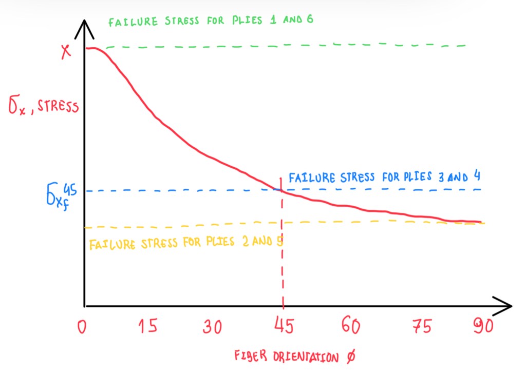
Moreover the failure stress are obtained through a failure criteria. In Figure 2, it is possible to notice that, the value of strength for 90° plies for any type of failure criteria is very low. For 0° plies, the strength is the highest one. In the case of 45° plies, it should be determined what is the failure strength for a wall index direction. This is determined by one of those failure criteria for the plies. Hence, this is a value which is dependent of the orientation of the ply. Therefore, the failure will occur into the plies oriented at 90°, then the ones at 45° and 0°, then in this example the first ply failure is the one at 90°.

Progressive ply failure example

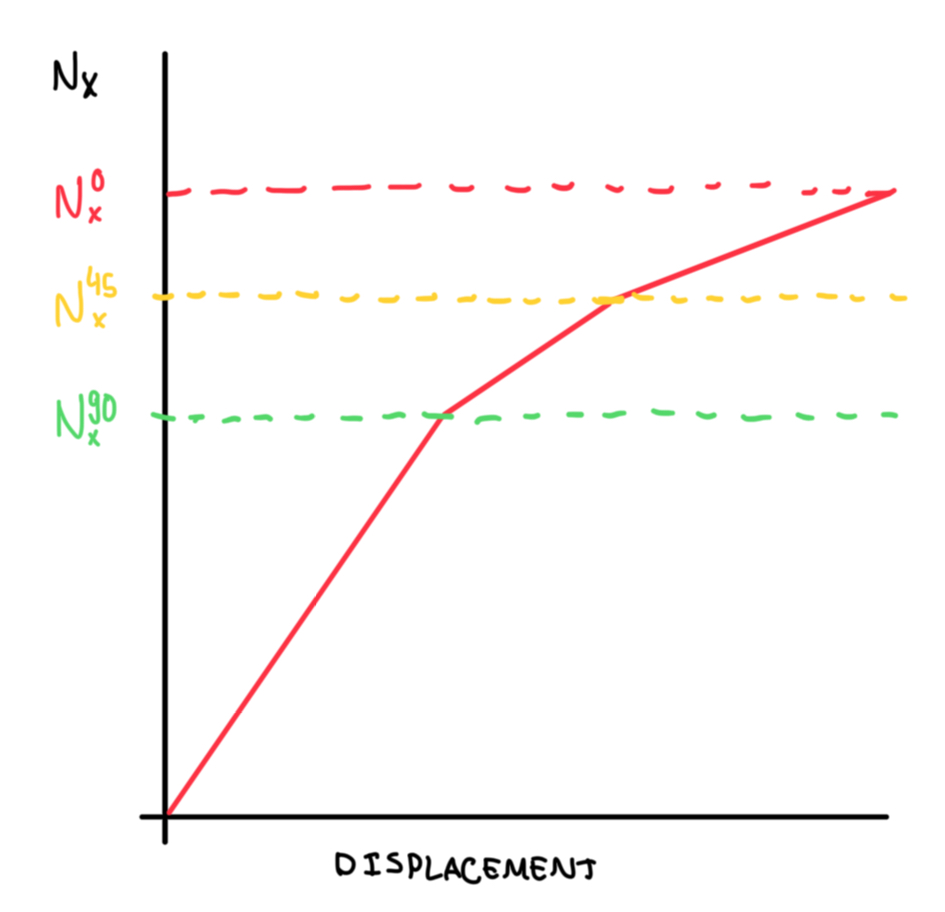
Figure 3 illustrates the same symmetric laminate exposed to a load Nx, but the failure criteria is the progressive one. In this case, it is important to check what happens after the failure of the plies at 90°. First, the loads are re-distributed and the values of N_x^45° and N_x^0° will change with respect to the previous one. The reason is due to the value of the matrix A, that changes from A” to A”‘, which are calculated after the failure of the plies at 90° and 45° plies. Hence, also the coefficients A” and A”‘ will change in the subsequent step, because they will not carry any load. The thickness of the laminate remains the same, because the laminate does not shrink. What only changes is the material stiffness matrix, which will not be miscalculated. Hence, for 90° plies and then for 45° plies after, this material stiffness matrix will be zero. Therefore, for the failure calculation, it will be taken into account the stiffness of 90° and 45° plies. This changes the stiffness of the laminate and results in a different final value for the strength. A’ is a coefficient of the A matrix when the plies are virgin or undamaged ones. A” is the coefficient when there is a laminate with just a 0° and 45° fibers, but with the elimination of 90° fibers without collapsing the laminate. Then A”‘ is the same coefficient as A”, but zeroing 90° and 45° fibers. Therefore, progressive ply failure is something done with the support of FEM. This accounts progressively the decrease in the stiffness and the strength. Then, in principle, this last failure might be even lower than the first ply failure one. However, since the special of the value of 0° plies is larger than the one of 90° plies, it is likely that this strength is larger than this one, but it is not possible to define which principle is larger or not.

Failure Envelope

For instance, the case illustrated in Figure 4 is a laminate where each 0°, 45° and 90° plies there is the failure envelope in terms of in-plane deformations (ε1, ε2) for different orientation of loading. There is a region enclosed between 0° and 90°, which is a safety region. It means that, the first ply failure will occur depending on the orientation angle given by failure of 90° or 0° plies. If the load is oriented in this way, the failure occurs by the angle of these plies. As long the plies are rotated, these will become a 0° ones. 45° plies will never be the first to failure. Or at least, there is one point where all those plies may fail at the same time. The last ply failure condition (Figure 4) is represented by those three sets of data, depending on the rotation load. It is possible to notice that for LPF, the safety region is enclosed by these sets of data. In addition, in the quadrant of the positive value of (ε1,ε2), there are loads that go from the direction 1 to the direction 2 and the last ply failure load is higher than the first ply failure one. Hence, there is a correlation failure. In the quadrant (+ε1,+ε2), the last ply failure load occurs before the first ply failure one. This means that, as soon that a source ply occurs, the laminate collapses. This is the reason why it can not be assumed in principle that, this last load is always higher than the first ply failure one. The last ply failure load depends on the orientation, the material strength and the lamination. There are load orientations that cause a progression of the failure, while there are others that cause the sum of the failure, thus the collapse of the laminate.

The total envelope is just the sum of these two (Figure 5), which means that the safety region is the one highlighted in Figure 5. This is a bit larger, specially in the quadrant (-ε1,-ε2) with respect to the first ply failure. Then with the first ply failure envelope, it can be shrinked whenever is necessary in order to define a certain margin. The safety margin is inside, thus if it is desired to have a specific one, then a limit should be placed. This limit is just a proportional shrinkage of the failure region. If it is taken a line from zero to cross the limit failure and goes until the outer limit, it is defined the safety margin highlighted in red.

Comparison between ply failure criteria

The comparison between the ply failure criteria can be seen in Figure 6. The main point is, that there are no overall more conservative criteria between these. The max stress theory exhibit a rectangular boundary that almost encloses all criteria. The interactive theory refer to Tsai-Hill or Tsai-Wu criteria, thus this make the other regions an interactive theory. The Tsai-Wu is maybe more conservative than the Max Stress Theory in some regions, while in the other, the Max Stress Theory is the more conservative one. Hence, it is difficult to define one of those criteria as the more conservative one. This is not the case for the isotropic material, for instance. In this example, it is always more conservative than the Max Stress Theory, which is not the case for composites.

Failure of notched laminates

A notch is a certain type of geometrical discontinuity, that can be a hole. The variation on the diameter for homogeneous materials is given by a coefficient, which deliver the stress along the notch as function of the stress due to the applied loading. For homogeneous isotropic materials, it is easier to calculate those coefficients, which is not the case for the anisotropic ones. In this case, there is a solution for Kt in a simple plate as illustrated by Figure 7.

In this case, the local stress at the notch is determined as Kt•σ (Figure 8). Kt depends on some terms of the sub-matrix A. The value of K_t in Figure 8 is from symmetric laminates. In addition, it is possible to notice that the value for isotropic material is 3, while the same for a T300 carbon-epoxy is 6.86. This is more than twice for the isotropic materials. The reason is that, the T300 carbon-epoxy unevenness of the stiffness in different directions. It is much more stiff in load direction, than it transverse directions. This causes to Kt has a higher impact. In the case of a different composite as S-glass ones, Kt is different because the stiffness in the fiber and in the transverse directions are similar, thus Kt is higher than T300 carbon-epoxy. Hence, Kt becomes dependent on the material stiffness. There is another value that is important to underline. This is the quasi-isotropic configuration [0°/90°/±45°], which is the only one that is independent from the stiffness on the fiber and at the transversal direction. These have variations from T300 carbon-epoxy and S-glass-epoxy. Both exhibit a Kt = 3, a value which is equal to the one for isotropic material. The quasi-isotropic delivers stiffnesses which are even on the same two in-plane directions, thus the laminate has the same stiffness on different directions as in isotropic materials. This is why this is considered as independent of the material, because when Kt is computed, there are terms that eliminates each other. For any other type of sequence, Kt value is dependent on the lay-up and material.

In the example in Figure 9, the impact of the hole radius was superimposed by the plate width, which is much higher than the hole. However, the hole radius has some influence. Figure 9 illustrates the effects of different diameters, at least qualitatively. In this example, there are four different combinations of the same material. These are 0°/±45°/90° plies, which are represented by the sequence of, for example, 50% of 0° plies, 40% of ±45° plies and 10% of 90° plies. This configuration is represented by the circle and the black dot. This laminate has 25 different plies. In addition, there are two different diameters, 1 and 0.25 inch. If it is considered the ratio between the strain and the allowable strain equals to 1, this means that the strains is equal to the strain of an unotched specimen. Depending on the hole size and the relative percentage of different plies orientations inside the laminate, it is possible to get values of strain. As lower is the diameter, higher is the failure strain at the notch root. In addition, for the same diameter, but having more 0° plies, a higher failure strain is obtained. To overcome this notch efffect, there is an evidence that performing several tests with different diameters and calculating the strain at certain distance from the notch root (strain that corresponds to the failure at the notch root), it is obtained the characteristic point of the material. The reason is that, if it is taken the strain at this point, it will be independent from the diameter and the laminate. Due to the notch effect, the values at the notch root are higher, then the difference in failure strength is smaller than expected. The reason is that, the failure strength measured is not one at the notch root. Actually, this is difficult to be measured since it requires strain-gauges. The strength measured is the total strength applied to the component, which is more or less given by the strength at a very far distance from the notch root. Hence, it is possible to consider that, this value is the strength of a failure measured in a tensile test machine. The fact that, the shift occurs depending on the hole diameter and the lay-up means that, the failure strength measured in a tensile testing is lower than expected. However, it is possible to notice that, a lower diameter hole have a lower failure strain, but the failure strength at notch root is higher than expected. This is influenced by the diameter.

The reason is not so intuitive since it is referred to the micro-structure and the probability in finding a defect on it. For example, Figure 10 highlights two different situations, which one of holes has a bigger diameter with respect to the other one. A smaller hole has a region where the strain are very high that captured a couple of fibers. In the case of a bigger hole, then there is also a region of high stresses, which is larger and takes more fibers. Hence, to occur the failure of the fibers on this region, a failure at micro-scale due to the presence of little defects on the matrix or the fibers must occur. Then there is a certain probability P1 to have a defect which is critical for the structure. In the case of a larger hole (d2), the region affected is bigger. This is the one that suffer from stresses above 95% of the maximum value. Hence, the smaller region has a probability P1 to find a critical defect, while the larger region has a probability P2. Since this probability is dependent of the volume on which it is calculated, P1 < P2. This means that, the larger the hole, the higher the probability to find a critical defect. This is the reason why the allowable strain of an unotched laminate is lower than the strain at failure in an unotched laminate. The volume of the region is proportional to the hole, that is the reason that there is notch effect, which is a special case of the size effect of strain. The larger the component, the larger is the volume which is stressed over a constant value and the higher is the probability to find a critical failure. There are probability theories which are based in the weakest link concept. This explains in mathematical terms the notch effect. The smaller is the notch, the larger is the effect on the global failure. However, the effect is lower than expected (Figure 10). Hence, the notch effect is not something that states that, a notched component will resist more than an unotched one. Actually, the notch effect states that a notched component is impaired in strain and stress of failure by an amount which is less than expected. If the stresses are calculated by the four different combinations (Figure 9 and 11) starting from the point where there is a failure strain at the notch, it is possible to get that all those combinations will collapse at a value of 1 at a certain distance. This is called characteristic length, which can be seen as a property of the material. The reason is that, if a test is performed on this length, then it is necessary just one test with the hole diameter to know that all the other tests will pass. Hence, it is just necessary to simulate all the other combinations to know the notch strain and the remote strain at failure. In general, a small hole motivates a high stress concentration, but the difference between the effect from a big and small hole is less than expected.

This can be seen on curve traces of Figure 11. For instance, the gray curve is related to a case that account only stress concentrations without notch effect. The notch is sometimes called, support, because it gives some rise of the curve with respect to the theoretical one. Hence, it always have some effect of the stress concentration which is not only given by the stress concentration factor, but it is necessary to account the notch effect, which it goes in the opposite direction. Hence, the smaller the hole, the higher the stress concentration and the higher the notch effect. The stress concentration decreases the failure strength, while the notch effect decreases the failure strain. At the end, if just one of these is considered, the approach will be a too conservative design. The notched structure can resist much more than expected. This concept is not so intuitive, because in general, the higher the stress, the lower the strength. The notch effect, in general, is also valid for other components. Metals, for instance, can exhibit, for small and large components, a fatigue resistance which is higher for the small parts with the same type of loading and maximum stress. There is a micromechanical reason, that if accounted, it maybe wrong for the same side of from the box.

Delamination failure

The delamination failure is a failure criteria that accounts the out-of-phase stresses and strain. Hence, it is necessary to know the out-of-plane stresses, which are not so straigthforward as the in-plane ones. The second point is the calculation of the interlaminar stresses. Since these are not constant, they are very dependent on their position on the interface. Some interlaminar stresses are higher when they are closer to the edge of the laminate. Hence, it is necessary to average them to get a valuer over a certain thickness. There are indications about its distance, for instance, if it is at twice ply thickness. Another indication is about how accounting the shear strength. The out-of-plane shear strength is considered as an in-plane shear strength, while the out-of-plane beam shear strength is taken as the transverse shear strength of the laminate.

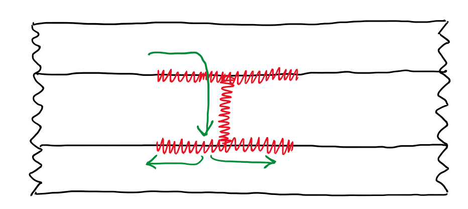
It is possible to have a control over the delamination, but this is often a consequence of a failure inside the ply. Hence, if there is a failure on the matrix at a certain point, it is developed delamination at the other plies. Figure 13 illustrates a series of plies. A crack develops in one ply, then it is likely that delamination develops in the edge of plies starting from that laminate. This means that, the delamination is not the first failure mechanism of failure. This is the reason why the delamination failure is not often studied, just in case of which is desired to monitor the progression of the delamination inside the laminate.

References

• Mallick, P.K. Fiber-Reinforced Composite: materials, manufacturing and design. Edition 3, CRC Press, 2008;
• This article was based on the lectures notes written by the author during the Design of Composite Materials for Racing Cars lectures attended at Università di Modena e Reggion Emilia.