The cover Figure illustrates that the grip is a function of, at least, F_Z, α and t. The slip angle α at the peak of grip is a function F_Z, though. This is a bit non intuitive, because the peak of sliding occurs at μ_k, which is lower than μ_s. The potential not used is higher than the amount lost when the tire pass from μ_s to μ_k. In addition, due to F_Z distribution and to the fact that friction is a local property, the grip is a third order parameter. Hence, the peak of grip is not μ_k*F_Z neither μ_s*F_Z. Instead, it is:

The portion of grip which is gained is higher than the one which is lost when it goes from μ_s to μ_k , as can be seen in the Figure 2:

This transition occurs along the contact patch length. At some point, the contact patch is under slip and sliding. This is the best condition, because the friction is neither at slip nor at sliding and the force produced is higher than the one at these conditions. This is confirmed by F_Ymax formula at Figure 1.

The Figure 3 illustrates an ordinary situation which a Force F is applied and a friction force ƒ is generated. While the relation between these is linear, F is equal to ƒ. However, when F reaches a threshold value, a collapse occurs and it reduces to a lower condition. The transition values between these phases (Figure 4) is the one which is given by Figure 1.

Hence, it is possible to summarize some conclusions about the friction force obtained during the tire operation:

Therefore, a tire produces its maximum F_Y when it works at a critical condition which is not characterized by μ_k*F_Z neither μ_s*F_Z. Instead, it is something between these two, which is defined by μ_s, χ and F_Z. In addition, the contact patch is totally under sliding. When F_Z is further increased, the frictions collapses and the lateral load decreases to μ_k*F_Z.

Contact patch stress distribution

Figure 6 illutrates that there is a direct connection between the cornerning stiffness C_S and tire contact patch area. It is possible to have two tires, a narrow and a wide one and these have the same contact patch area. In addition, these tires are submitted to the same slip angle and they have the same construction. Since cornering stiffness is given by the equation above, the main parameter relative to contact patch is its length, thus these tires will have different C_S, which means that for the same α, they generate different grip. Hence, the wider tire has to perform a higher α to produce the same F_Y than the narrower tire. In fact, the difference between tire dimensions go beyond C_S. Wider tires usually are more sensitive to camber variation than the narrow ones. However, narrow tires have more deformation of the contact patch to compensate the camber angle γ. In fact, the contact patch of a cambered tire is not squared, instead it is more trapezoidal. For this reason, cambered tires steer naturaly since there is always a lateral speed component (Figure 7).

This results in V_y due to γ. This component is added to α due to the lateral force produced. However, the component from γ acts differently, it creates a moment which makes the tire steer naturaly (Figure 8).

Finally, it is possible to understand that camber has some add to the lateral force. The F_y amount can change according to the type of the tire. In general, the ratio between camber and cornering stiffness is higher for cross-ply tires than the radial ones, 1/6 against 1/20, respectively.

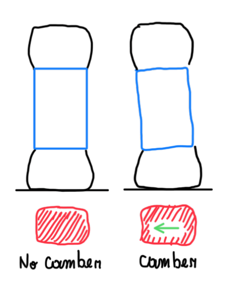
The trapezoidal contact patch occurs due to camber. For instance, tires used in oval racing have their sidewalls exposed to different stresses. The inner sidewall have a softer material relative to the outer sidewall.. Consequently, this is more compliant, because loads are lower, thus the stresses too.

Longitudinal loads

The longitudinal loads are exposed to the same theory about the bristle movements. As can be seen, there two zones along the contact line (brush model reduces the contact area into a line), the adhesion and the sliding ones. If it was possible to follow one bristle, would be possible to visualize its deformation during the movement until its detachment. In the Figure 10a, the bristle is attached to the surface and has no deformation. As the tire rotates, it deforms more and more, as seen in Figures 10b and 10c. However, at some point, the tip of the bristle goes from the adhesion to the sliding condition. In this case, the bristle continues to distort, but the tire rotate more and the bristle tip is detached from the surface.

Understanding that the tire is exposed to adhesion and slide conditions, when the tire is under combined loads, F_Y and F_X together, the total force produced by the tire is a combination of adhesion and sliding. However, this condition is not present in the beginning. The tire is basically at adhesion state in the beginning of movement. As soon the loads increase, some bristles enter in the sliding condition, as can be seen in the Figure 11a. As the total force increases, the slip coefficient σ variates from 0.04 until 0.26. However, the maximum tangential load occurs when σ is 0.20. The peak of total force is obtained at this condition, because these are occupied under the two curves (Figure 11c). When loads increase, σ increases, but now μ goes to μ_k. The energy produced in the contact is now under the kinetic friction force, which is the lowest one (Figure 11d).

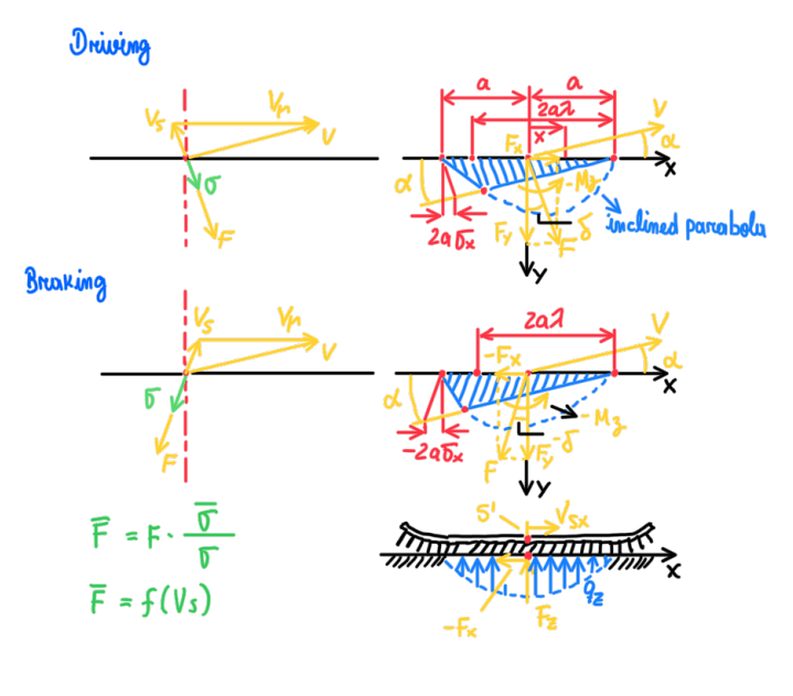
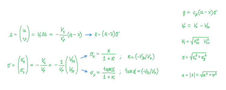
The main longitudinal movements are free rolling, driving and braking. The first one is characterized by the fact that the rolling radius is equal to the wheel radius. In addition, V_sx is zero, because there is no slip. In the case of driving and braking movements, there is some slip. Hence, r_e is different from r and V_sx is non zero. The slip results in the so called longitudinal deflection, given by the equations and formulas above (Figure 12). However, it is interesting to expand this information in terms of the slip coefficients σ_χ and σ_y and correlate them with tire composite parameter θ_y:

The lateral stiffness c_p is the only difference between θ_x and θ_y, which is essentially the belt characteristics, where c_px and c_py are the longitudinal and the lateral stiffness, respectively. In real condition, c_ƒx is approximately 1.5∙c_ƒy. This occurs because tires are anisotropic. They must deal with longitudinal and lateral forces. In addition, due to a 90° round shaped tread and the great concern to keep it as flat and as in contact as possible to the surface. The sidewalls and plies are built to generate this. Hence, the consequence is that c_ƒx = 1.5∙c_ƒy. The situation changes when tires are performing movements which generates low levels of deformations, thus the equations in the Figure 14 must be updated:

As can be seen, in this case, the longitudinal slip k and the slip angle α are so small, that the longitudinal and the lateral deflection are reduced to the difference between a and x times the slip parameter respective to these movements, σ_χ or σ_y.

Combined slip

The combined slip is a situation which both lateral and longitudinal loads are occurring at the same time. In these cases the effect of σ_χ and α are even more important. The equations for this case were already described in Figures 12, 13 and 14, but when these are combined with the system of equations they are thus characterized by vectors and matrices which differs according to the tire contact patch situation, adhesion or sliding. In the first case it can be written:

As can be seen in the Figure 16, in the adhesion case the vector e is simplified, because there is no slip, thus the terms referred to the relative speed and radius are neglected and equal to the nominal value, respectively. Moreover, it is possible to split the longitudinal and the lateral components of the combined deflection term e. Basically e is equal to the square of u and v (Figure 16). In the case of sliding tire contact patch condition, it can be written:

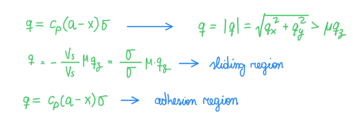
Therefore, the sliding condition in the combined slip (Figure 17) of the brush model is dependent of F_Z and µ. In addition, the ratio between the total theoretical slip coefficient and the lateral or the longitudinal ones defines the local stress produced during the combined slip movement (Figure 17).

Finally, with these equations (Figure 17) it is possible to visualize the effects of the longitudinal slip ratio k and the slip angle α in the main wheel loads, F_Y, F_X and M_Z. Fixing θ equal 5, it is possible to notice that during braking or driving, when F_Y is applied, the main effects comes from α . However, if k changes from values far from zero, which represents braking or driving situation, F_Y drastically reduces even if α is an ideal value. There is another detail which is better to observe at the friction circle (right graph from Figure 18). The braking side has a bigger radius relative to the driving side. Cars produce more longitudinal force when braking due to drag and load transfer. These factors increase the front tire F_Z, thus their grip. For this reason it is normal to observe that for the same modulus of the longitudinal slip ratio k, during combine braking, F_Y is higher. The lines of constant α form ellipses which are more deformed at the braking side due to k. In all cases, the increase of α produce more F_Y, but as k increases, either braking or driving, this capability to produce F_Y reduces. Therefore, this is the reason which is possible to turn-in during a heavy braking, while the same combined slip for driving generates a reduced turn-in capability (Figure 18).

The function of the steering angle to maintain the car under equilibrium. The handling is adjusted by the acceleration and braking pads. The driver demands the steering wheel to balance the conditions due to the accelerator or the braking pedal inputs. The main reason for this phenomena is that the longitudinal load transfer occurs in a much higher speed than the lateral load transfer. Therefore, the rate which the driver activates or deactivates the throttle or the braking pedal is critical to define which is the ideal steering angle for that situation. Moreover, oversteering and understeering is a consequence of the driver’s inputs. Hence, the equilibrium condition can be understeered or oversteered behavior of the car. The braking release speed tunes the vertical load on the front tires. Therefore, braking skills of the driver are the main technique to define handling. In other words, if the driver demands more F_X, then tires deliver less F_Y.

Reference

• Race Car Vehicle Dynamics – Miliken & Miliken;
• Guiggiani, Massimo. The Science of Vehicle Dynamics. Handling, Braking, and Ride of Road and Race Cars. New York, Springer, 2014;
• Haney, Paul. The Racing & High-Performance Tire – Using the Tires to Tune for Grip & Balance. TV Motorsports, SAE, January, 2003.