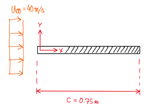
A flat plate has a chord c = 0.75 m, negligible thickness and a span wise length b = 1 m. It is immersed in an air flow with a free stream velocity U_∞ = 40 m/s. The x-axis is parallel to the air flow, while the y-axis is vertical to the stream velocity. The x = 0 coordinate coincides with leading edge of the flat plate and x = c coordinate coincides with trailing edge of the flat plate.

First part

In the first part of the exercise, the flat plate is displaced horizontally, thus α = 0 as seen at cover Figure.

Question 1 – Calculate the vorticity vector at the upper surface at point (c,0,0) understanding that the local friction coefficient is c_ƒ = 0.003

Re = U_∞∙x/υ = (40∙0.75)/(15∙10^-6) = 2000000 = 2∙10⁶ → Turbulent

ω = – ∂u/∂y ; τ_w = μ∙(∂u/∂y) → (∂u/∂y) = τ_w/μ

c_ƒ = τ_w/q_∞ → τ_w = c_ƒ∙q_∞

ω = – c_ƒ∙q_∞/μ = – (0.003∙960)/(18∙10^-6) = 160000 Pa/(Pa∙s) = 1.6∙10⁵ s^-1

As can be seen, the air flow has enough speed to be considered turbulent. The vorticity is known as – ∂u/∂y. However, it is obtained through the boundary layer friction since c_ƒ is already given and there is no velocity profile equation. Hence, it is possible to conclude that in this exercise the vorticity is basically proportional to the square of the free stream velocity.

Question 2 – Calculate the mass flow rate of the boundary layer in m²/s

Calculate q’ respective to (x = c , z = 0) and for y > 0 knowing that δ = 0.016 m and the boundary layer thickness is δ* = 0.002. This question is basically formula application, thus:

q’ = U_∞∙(δ – δ*) = 40∙(0.016 – 0.002) = 0.56 m²/s

Question 3 – Develop the analytical expression of the mass flow rate at (x = c , y > 0 , z = 0) for a given velocity profile

The velocity profile is given by:

This question asked about the analytical expression for the mass flow rate due to the displacement thickness. Since the velocity profile is given, it is just necessary to describe the boundary layer displacement thickness equation. At the end, it is possible to conclude that the flow rate is only proportional to the boundary layer thickness. The velocity profile and the displacement thickness only vary the degree of proportionality.

Second part

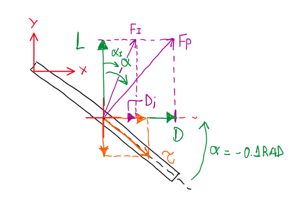
In the second part of the exercise, the flat plate exhibits an inclination α = – 0.1 rad and a lift behavior with L = 180 N without the viscous effects.

Question 4 – Estimate the induced drag considering the elliptical wing hypothesis

α_i = C_L/(π∙AR) → C_L = α_i∙π∙AR

cos(α_i) = L/F_i ; sin(α_i) = D_i/F_i ; F_i = L/cos(α_i) = D_i/sin(α_i)

D_i = L∙(sin(α_i)/cos(α_i)) = L∙tg(α_i)

L = CL∙q_∞∙S → CL = L/(q_∞∙S) = α_i∙π∙AR → α_i = L/(q_∞∙S∙π∙AR)

q_∞ =½∙ρ∙U_∞² = ½∙1.2∙40² = 960 Pa

S = 1∙0.75 = 0.75 m²

AR = b/c = 1/0.75

α_i = L/(q_∞∙S∙π∙AR) = 180/(960∙0.75∙(1/0.75)∙π) = 0.059683104 ≃ 0.059

D_i = L∙tgα_i = 180∙tg(0.059) = 10.756 N

It is important to remember that the lift L given is the lift component without the lift generated by the viscous force τ (Figure 1), this is L_ƒ = τ∙sin(α). As can be seen, the lift L, which was given, does not account the viscous force. If the total lift was asked, may the induced component would be useful.

Third part

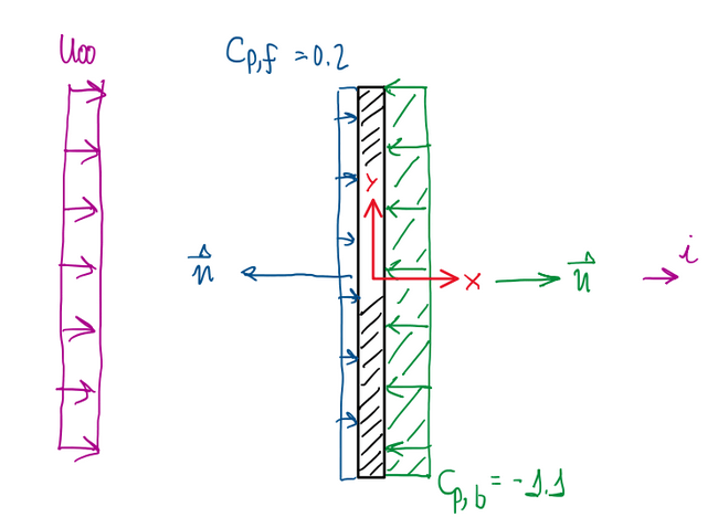
The third section of this exercise, the flat plate is perpendicular to the air flow, α = -π/2 rad. The drag coefficient C_D = 1.3 and the pressure coefficient at the base is C_P,b = -1.1.

Question 6 – Calculate the average pressure coefficient at the front C_P,f

Db = -q_∞∫C_P,b∙(n∙i)dS = -q_∞∙C_P,b∙c ; n∙i = 1

Df = -q_∞∫C_P,f∙(n∙i)dS = q_∞∙C_P,f∙c ; n∙i = -1

D = q_∞∙C_D∙c

D = D_f + D_b = q_∞∙C_D∙c = q_∞∙C_P,f∙c + (-q_∞∙C_P,b∙c)

q_∞∙C_D∙c = q_∞∙C_P,f∙c – -q_∞∙C_P,b∙c

C_D = C_P,f – C_P,b → C_P,f = C_D + C_P,b = 1.3 – 1.1 = 0.2

Question 7 – Calculate the energetic content of the wake generated by the flat plate per unit length

E₀‘ = D = q_∞∙C_D∙S = 960∙1.3∙1∙0.75 = 936 Nm/m

Conclusion

The main point of this exercise is the attack angle variation. Different from the other exercises, it was assumed that the flat plate behaves as an elliptic wing. This makes easier to find the induced angle α_i, because elliptic wing are the ones which the distribution of the circulation is elliptical and symmetrical along the wing span. Hence, it is quite straight forward to find α_i since L was given. What makes a bit confusing is that difference between α_i and α, which is illustrated at Figure. Understanding this, it is just application of geometrical and trigonometrical rules. Usually, these exercises assumes the simplification for very small angles.